In a recent post (and papers), Anders Huitfeldt and co-authors have discussed ways of achieving external validity in the presence of “effect heterogeneity.” These results are not immediately inferable using a standard (non-parametric) selection diagram, which has led them to conclude that selection diagrams may not be helpful for “thinking more closely about effect heterogeneity” and, thus, might be “throwing the baby out with the bathwater.”
Taking a closer look at the analysis of Anders and co-authors, and using their very same examples, we came to quite different conclusions. In those cases, transportability is not immediately inferable in a fully nonparametric structural model for a simple reason: it relies on functional constraints on the structural equation of the outcome. Once these constraints are properly incorporated in the analysis, all results flow naturally from the structural model, and selection diagrams prove to be indispensable for thinking about heterogeneity, for extrapolating results across populations, and for protecting analysts from unwarranted generalizations. See details in the full note.
This post introduces readers to Fréchet inequalities using modern visualization techniques and discusses their applications and their fascinating history.
Fréchet inequalities, also known as Boole-Fréchet inequalities, are among the earliest products of the probabilistic logic pioneered by George Boole and Augustus De Morgan in the 1850s, and formalized systematically by Maurice Fréchet in 1935. In the simplest binary case they give us bounds on the probability P(A,B) of two joint events in terms of their marginals P(A) and P(B):
The reason for revisiting these inequalities 84 years after their first publication is two-fold:
They play an important role in machine learning and counterfactual reasoning (Ang and Pearl, 2019)
We believe it will be illuminating for colleagues and students to see these probability bounds displayed using modern techniques of dynamic visualization
Fréchet bounds have wide application, including logic (Wagner, 2004), artificial intelligence (Wise and Henrion, 1985), statistics (Rüschendorf, 1991), quantum mechanics (Benavoli et al., 2016), and reliability theory (Collet, 1996). In counterfactual analysis, they come into focus when we have experimental results under treatment (X = x) as well as denial of treatment (X = x’) and our interests lie in individuals who are responsive to treatment, namely those who will respond if exposed to treatment and will not respond under denial of treatment. Such individuals carry different names depending on the applications. They are called compliers, beneficiaries, respondents, gullibles, influenceable, persuadable, malleable, pliable, impressionable, susceptive, overtrusting, or dupable. And as the reader can figure out, the applications in marketing, sales, recruiting, product development, politics, and health science is enormous.
Although narrower bounds can be obtained when we have both observational and experimental data (Ang and Pearl, 2019; Tian and Pearl, 2000), Fréchet bounds are nevertheless informative when it comes to concluding responsiveness from experimental data alone.
Plots
Below we present dynamic visualizations of Fréchet inequalities in various forms for events A and B. Hover or tap on an ⓘ icon for a short description of each type of plot. Click or tap on a type of plot to see an animation of the current plot morphing into the new plot. Hover or tap on the plot itself to see an informational popup of that location.
ⓘⓘⓘⓘⓘ
ⓘⓘⓘⓘⓘ
The plots visualize probability bounds of two events using logical conjunction, P(A,B), and logical disjunction, P(A∨B), with their marginals, P(A) and P(B), as axes on the unit square. Bounds for particular values of P(A) and P(B) can be seen by clicking on a type of bounds next to conjunction or disjunction and tracing the position on the plot to a color between blue and red. The color bar next to the plot indicates the probability. Clicking a different type of bounds animates the plot to demonstrate how the bounds changes. Hovering over or tapping on the plot reveals more information about the position being pointed at.
The gap between upper bounds and lower bounds gets vanishingly narrow near the edges of the unit square, which means that we can accurately determine the probability of the intersection given the probability of the marginal probabilities. The range plots make this very clear and they are the exact same plots for both P(A,B) and P(A∨B). Notice that the center holds the widest gaps. Every plot is symmetric around the P(B) = P(A) diagonal, this should be expected as P(A) and P(B) play interchangeable rolls in Fréchet inequalities.
Example 1 – Chocolate and math
Assume you measure the probabilities of your friends liking math and liking chocolate. Let A stand for the event that a friend picked at random likes math and B for the event that a friend picked at random likes chocolate. It turns out P(A) = 0.9 (almost all of your friends like math!) and P(B) = 0.3. You want to know the probability of a friend liking both math and chocolate, in other words you want to know P(A,B). If knowing whether a friend likes math doesn’t affect the probability they like chocolate, then events A and B are independent and we can get the exact value for P(A,B). This is a logical conjunction of A and B, so next to “Conjunction” above the plot, click on “Independent.” Trace the location in the plot where the horizontal axis, P(A), is at 0.9 and the vertical axis, P(B), is at 0.3. You’ll see P(A,B) is about 0.27 according to the color bar on the right.
However, maybe enjoying chocolate makes it more likely you’ll enjoy math. The caffeine in chocolate could have something to do with this. In this case, A and B are dependent and we may not be able to get an exact value for P(A,B) without more information. Click on “Combined” next to “Conjunction”. Now trace (0.9,0.3) again on the plot. You’ll see P(A,B) is between 0.2 and 0.3. Without knowing how dependent A and B are, we get fairly narrow bounds for the probability a friend likes both math and chocolate.
Example 2 – How effective is your ad?
Suppose we are conducting a marketing experiment and find 20% of customers will buy if shown advertisement 1, while 45% will buy if shown advertisement 2. We want to know how many customers will be swayed by advertisement 2 over advertisement 1. In other words, what percentage of customers buys if shown advertisement 2 and doesn’t buy when shown advertisement 1? To see this in the plot above, let A stand for the event that a customer won’t buy when shown advertisement 1 and B for the event that a customer will buy when shown advertisement 2: P(A) = 100% – 20% = 80% = 0.8 and P(B) = 45% = 0.45. We want to find P(A,B). This joint probability is logical conjunction, so click on “Lower bounds” next to “Conjunction.” Tracing P(A) = 0.8 and P(B) = 0.45 lands in the middle of the blue strip corresponding to 0.2 to 0.3. This is the lower bounds, so P(A,B) ≥ 0.25. Now click on “Upper bounds” and trace again. You’ll find P(A,B) ≤ 0.45. The “Combined” plot allows you to visualize both bounds at the same time. Hovering over or tapping on location (0.8,0.45) will display the complete bounds on any of the plots.
We might think that exactly 45% – 20% = 25% of customers were swayed by advertisement 2, but the plot shows us a range between 25% and 45%. This is because some people may buy if shown advertisement 1 and not buy if shown advertisement 2. As an example, if advertisement 2 convinces an entirely different segment of customers to buy than advertisement 1 does, then none of the 20% of customers who will buy after seeing advertisement 1 would buy if they had seen advertisement 2 instead. In this case, all 45% of the customers who will buy after seeing advertisement 2 are swayed by the advertisement.
Example 3 – Who is responding to treatment?
Assume that we conduct a controlled randomized experiment (CRT) to evaluate the efficacy of some treatment X on survival Y, and find no effect whatsoever. For example, 10% of treated patients recovered, 90% died, and exactly the same proportions were found in the control group (those who were denied treatment), 10% recovered and 90% died.
Such treatment would no doubt be deemed ineffective by the FDA and other public policy makers. But health scientists and drug makers might be interested in knowing how the treatment affected individual patients: Did it have no effect on ANY individual or, perhaps, cured some and killed others. In the worst case, one can imagine a scenario where 10% of those who died under treatment would have been cured if not treated. Such a nightmarish scenario should surely be of grave concern to health scientists, not to mention patients who are seeking or using the treatment.
Let A stand for the event that patient John would die if given the treatment and B for the event that John would survive if denied treatment. The experimental data tells us that P(A) = 90% and P(B) = 10%. We are interested in the probability that John would die if treated and be cured if not treated, namely P(A,B).
Examining plot 1 we find that P(A,B), the probability that John is among those adversely reacting to the treatment is between zero and 10%. Quite an alarming finding, but not entirely unexpected considering the fact that randomized experiments deal with averages over populations and do not provide us information about an individual’s response. We may wish to ask what experimental results would assure John that he is not among the adversely affected. Examining the “Upper bound” plot we see that to guarantee a probability less than 5%, either P(A) or P(B) must be lower than 5%. This means that the mortality rate under either treatment or no-treatment should be lower than 5%.
Inequalities
In mathematical notation, the general Fréchet inequalities take the form:
If events A and B are independent, then we can plot exact values:
P(A,B) = P(A)·P(B)
P(A∨B) = P(A) + P(B) – P(A)·P(B)
Maurice Fréchet
Maurice Fréchet was a significant French mathematician with contributions to topology of point sets, metric spaces, statistics and probability, and calculus (Wikipedia Contributors, 2019). Fréchet published his proof for the above inequalities in the French journal Fundamenta Mathaticae in 1935 (Fréchet, 1935). During that time, he was Professor and Chair of Differential and Integral Calculus at the Sorbonne (Sack, 2016).
Jacques Fréchet, Maurice’s father, was the head of a school in Paris (O’Connor and Robertson, 2019) while Maurice was young. Maurice then went to secondary school where he was taught math by the legendary French mathematician Jacques Hadamard. Hadamard would soon after become a professor at the University of Bordeaux. Eventually, Hadamard would become Fréchet’s advisor for his doctorate. An educator like his father, Maurice was a schoolteacher in 1907, a lecturer in 1908, and then a professor in 1910 (Bru and Hertz, 2001). Probability research came later in his life. Unfortunately, his work wasn’t always appreciated as the renowned Swedish mathematician Harald Cramér wrote (Bru and Hertz, 2001):
“In early years Fréchet had been an outstanding mathematician, doing pathbreaking work in functional analysis. He had taken up probabilistic work at a fairly advanced age, and I am bound to say that his work in this field did not seem very impressive to me.”
Nevertheless, Fréchet would go on to become very influential in probability and statistics. As a great response to Cramér’s former criticism, an important bound is named after both Fréchet and Cramér, the Fréchet–Darmois–Cramér–Rao inequality (though more commonly known as Cramér–Rao bound)!
History
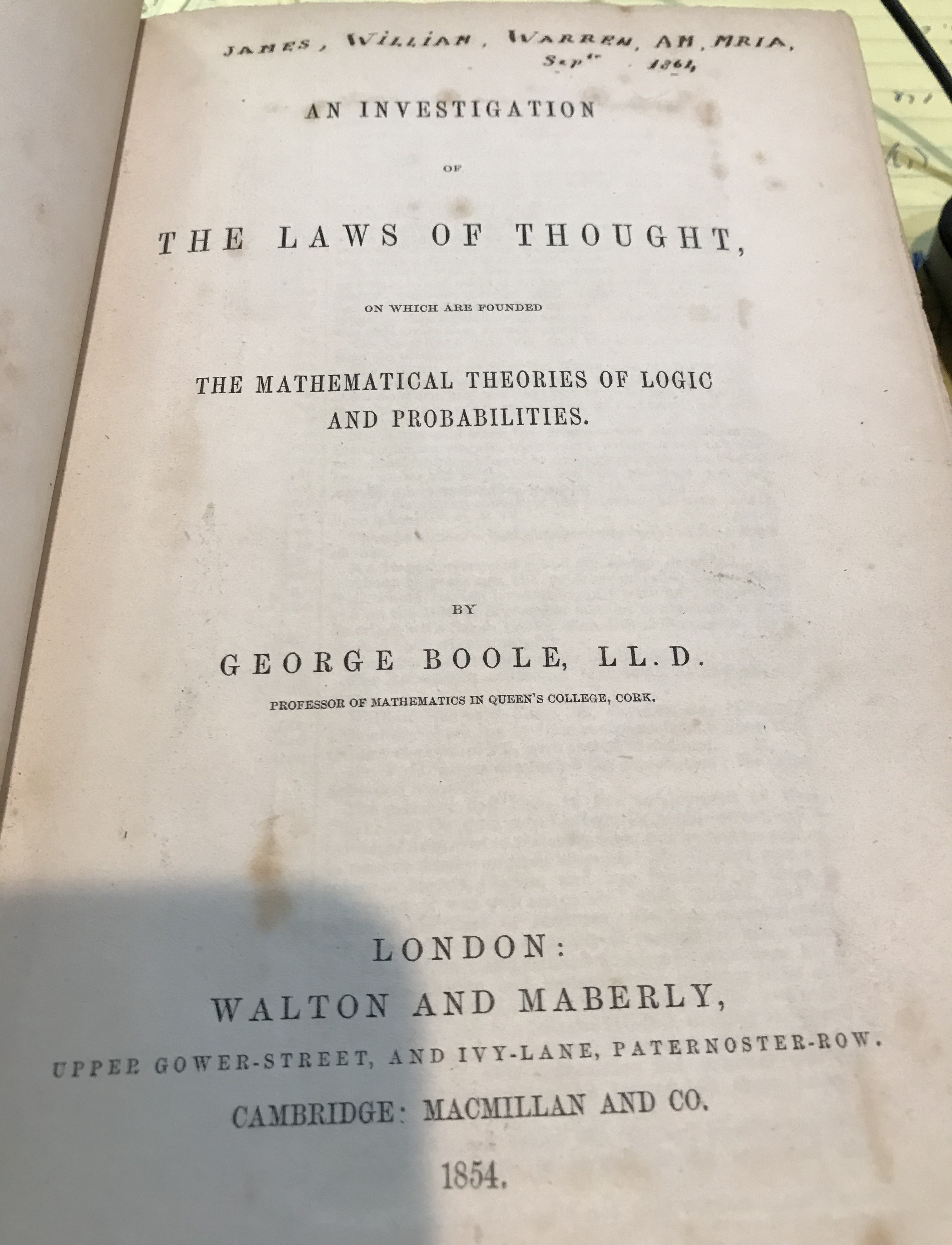
The reason Fréchet inequalities are also known as Boole-Fréchet inequalities is that George Boole published a proof of the conjunction version of the inequalities in his 1854 book An Investigation of the Laws of Thought (Boole, 1854). In chapter 19, Boole first showed the following:
Major limit of n(xy) = least of values n(x) and n(y) Minor limit of n(xy) = n(x) + n(y) – n(1).
The terms n(xy), n(x), and n(y) are the number of occurrences of xy, x, and y, respectively. The term n(1) is the total number of occurrences. The reader can see that dividing all n-terms by n(1) yields the binary Fréchet inequalities for P(x,y). Boole then arrives at two general conclusions:
1st. The major numerical limit of the class represented by any constituent will be found by prefixing n separately to each factor of the constituent, and taking the least of the resulting values. 2nd. The minor limit will be found by adding all the values above mentioned together, and subtracting from the result as many, less one, times the value of n(1).
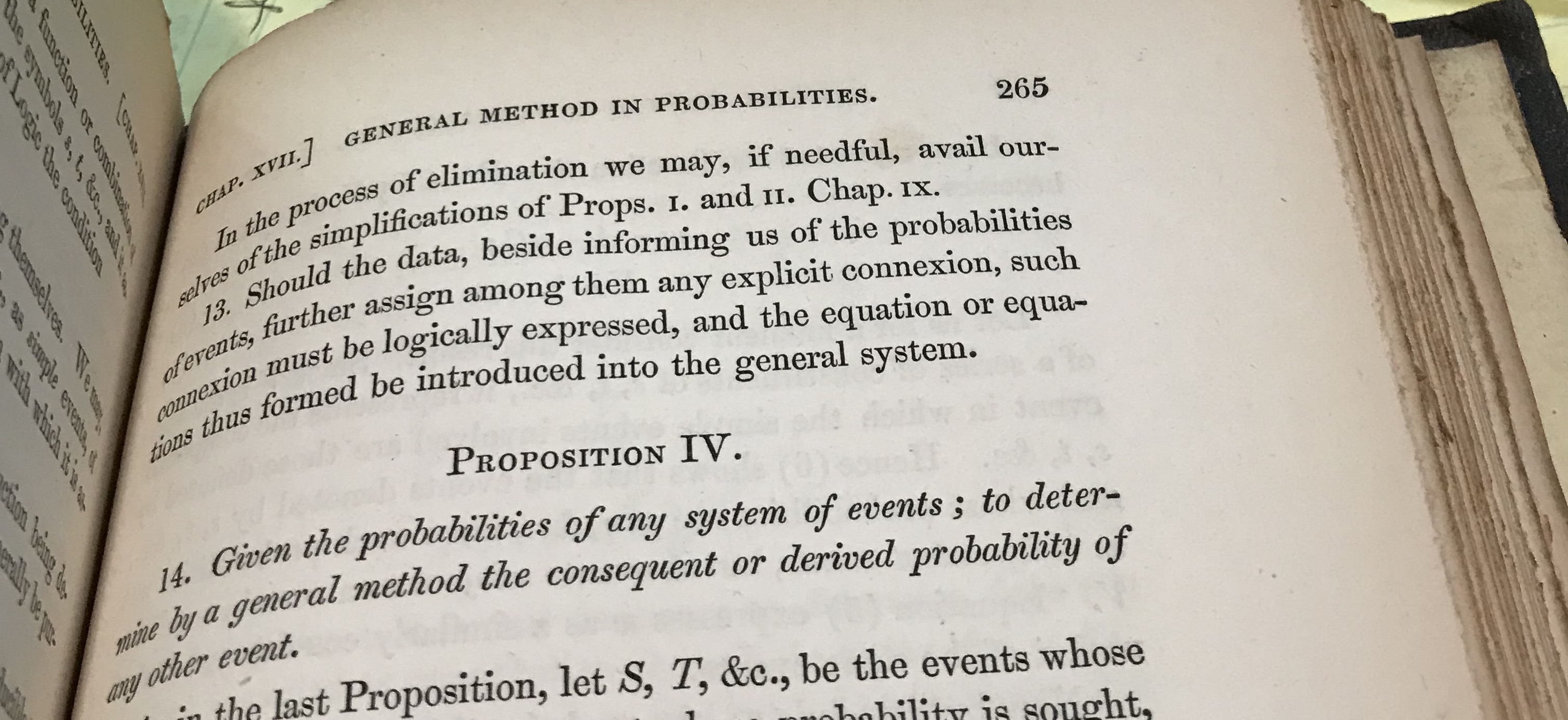
This result was an exercise that was part of an ambitious scheme which he describes in “Proposition IV” of chapter 17 as:
Given the probabilities of any system of events; to determine by a general method the consequent or derived probability of any other event.
We know now that Boole’s task is super hard and, even today, we are not aware of any software that accomplishes his plan on any sizable number of events. The Boole-Fréchet inequalities are a tribute to his vision.
Boole’s conjunction inequalities preceded Fréchet’s by 81 years, so why aren’t these known as Boole inequalities? One reason is Fréchet showed, for both conjunction and disjunction, that they are the narrowest possible bounds when only the marginal probabilities are known (Halperin, 1965).
Boole wrote a footnote in chapter 19 of his book that Augustus De Morgan, who was a collaborator of Boole’s, first came up with the minor limit (lower bound) of the conjunction of two variables:
the minor limit of nxy is applied by Professor De Morgan, by whom it appears to have been first given, to the syllogistic form: Most men in a certain company have coats. Most men in the same company have waistcoats. Therefore some in the company have coats and waistcoats.
De Morgan wrote about this syllogism in his 1859 paper “On the Syllogism, and On the Logic of Relations” (De Morgan, 1859). Boole and De Morgan became lifelong friends after Boole wrote to him in 1842 (Burris, 2010). Although De Morgan was Boole’s senior and published a book on probability in 1835 and on “Formal Logic” in 1847, he never reached Boole’s height in symbolic logic.
Predating Fréchet, Boole, and De Morgan is Charles Stanhope’s Demonstrator logic machine, an actual physical device, that calculates binary Fréchet inequalities for both conjunction and disjunction. Robert Harley wrote an article in 1879 in Mind: A Quarterly Review of Psychology and Philosophy (Harley, 1879) that described Stanhope’s instrument. In addition to several of these machines having been created, Stanhope had an unfinished manuscript of logic he wrote between 1800 and 1815 describing rules and construction of the machine for “discovering consequences in logic.” In Stanhope’s manuscript, he describes calculating the lower bound of conjunction with α, β, and μ, where α and β represent all, some, most, fewest, a number, or a definite ratio of part to whole (but not none), and μ is unity: “α + β – μ measures the extent of the consequence between A and B.” This gives the “minor limit.” Some examples are given by Harley. One of them is that some of 5 pictures hanging on the north side and some of 5 pictures are portraits tells us nothing about how many pictures are portraits hanging in the north. But if 3/5 are hanging in the north and 4/5 are portraits, then at least 3/5 + 4/5 – 1 = 2/5 are portraits on the north side. Similarly, with De Morgan’s coats syllogism, “(most + most – all) men = some men” have both coats and waistcoats.
The Demonstrator logic machine works by sliding red transparent glass from the right over a separate gray wooden slide from the left. The overlapping portion will look dark red. The slides represent probabilities, P(A) and P(B), where sliding the entire distance of the middle square represents a probability of 1. The reader can verify that the dark red (overlap) is equivalent to the lower bound, P(A) + P(B) – 1. To find the “major limit,” or upper bound, simply slide the red transparent glass from the left on top of the gray slide. Dark red will appear as the length of the shorter of the two slides, min{P(A), P(B)}!
Ang Li and Judea Pearl, “Unit Selection Based on Counterfactual Logic,” UCLA Cognitive Systems Laboratory, Technical Report (R-488), June 2019. In Proceedings of the Twenty-Eighth International Joint Conference on Artificial Intelligence (IJCAI-19), 1793-1799, 2019. [Online]. Available: http://ftp.cs.ucla.edu/pub/stat_ser/r488-reprint.pdf. [Accessed Oct. 11, 2019].
Carl G. Wagner, “Modus tollens probabilized,” Journal for the Philosophy of Science, vol. 55, pp. 747–753, 2004. [Online serial]. Available: http://www.math.utk.edu/~wagner/papers/2004.pdf. [Accessed Oct. 7, 2019].
Ben P. Wise and Max Henrion, “A Framework for Comparing Uncertain Inference Systems to Probability,” In Proc. of the First Conference on Uncertainty in Artificial Intelligence (UAI1985), 1985. [Online]. Available: https://arxiv.org/abs/1304.3430. [Accessed Oct. 7, 2019].
L. Rüschendorf, “Fréchet-bounds and their applications,” Advances in Probability Distributions with Given Marginals, Mathematics and Its Applications, pp. 151–187, 1991. [Online]. Available: https://books.google.com/books?id=4uNCdVrrw2cC. [Accessed Oct. 7, 2019].
Alessio Benavoli, Alessandro Facchini, and Marco Zaffalon, “Quantum mechanics: The Bayesian theory generalised to the space of Hermitian matrices,” Physics Review A, vol. 94, no. 4, pp. 1-26, Oct. 10, 2016. [Online]. Available: https://arxiv.org/abs/1605.08177. [Accessed Oct. 7, 2019].
J. Collet, “Some remarks on rare-event approximation,” IEEE Transactions on Reliability, vol. 45, no. 1, pp. 106-108, Mar 1996. [Online]. Available: https://ieeexplore.ieee.org/document/488924. [Accessed Oct. 7, 2019].
Maurice Fréchet, “Généralisations du théorème des probabilités totales,” Fundamenta Mathematicae, vol. 25, no. 1, pp. 379–387, 1935. [Online]. Available: http://matwbn.icm.edu.pl/ksiazki/fm/fm25/fm25132.pdf. [Accessed Oct. 7, 2019].
Harald Sack, “Maurice René Fréchet and the Theory of Abstract Spaces,” SciHi Blog, Sept. 2016. [Online]. Available: http://scihi.org/maurice-rene-frechet/. [Accessed Oct. 7, 2019].
George Boole, An Investigation of the Laws of Thought on Which are Founded the Mathematical Theories of Logic and Probabilities, Cambridge: Macmillan and Co., 1854. [E-book] Available by Project Gutenberg: https://books.google.com/books?id=JBbkAAAAMAAJ&pg=PA201&lpg=PA201. [Accessed Oct. 11, 2019].
Theodore Hailperin, The American Mathematical Monthly, vol. 72, no. 4, pp. 343-359, April 1965. [Abstract]. Available: https://www.jstor.org/stable/2313491. [Accessed Oct. 11, 2019].
Jin Tian and Judea Pearl, “Probabilities of causation: Bounds and identification.” In Craig Boutilier and Moises Goldszmidt (Eds.), Proceedings of the Conference on Uncertainty in Artificial Intelligence (UAI-2000), San Francisco, CA: Morgan Kaufmann, 589–598, 2000. Available: http://ftp.cs.ucla.edu/pub/stat_ser/R271-U.pdf. [Accessed Oct. 31, 2019].
If you were trained in traditional regression pedagogy, chances are that you have heard about the problem of “bad controls”. The problem arises when we need to decide whether the addition of a variable to a regression equation helps getting estimates closer to the parameter of interest. Analysts have long known that some variables, when added to the regression equation, can produce unintended discrepancies between the regression coefficient and the effect that the coefficient is expected to represent. Such variables have become known as “bad controls”, to be distinguished from “good controls” (also known as “confounders” or “deconfounders”) which are variables that must be added to the regression equation to eliminate what came to be known as “omitted variable bias” (OVB).
Recent advances in graphical models have produced a simple criterion to distinguish good from bad controls, and the purpose of this note is to provide practicing analysts a concise and visible summary of this criterion through illustrative examples. We will assume that readers are familiar with the notions of “path-blocking” (or d-separation) and back-door paths. For a gentle introduction, see d-Separation without Tears.
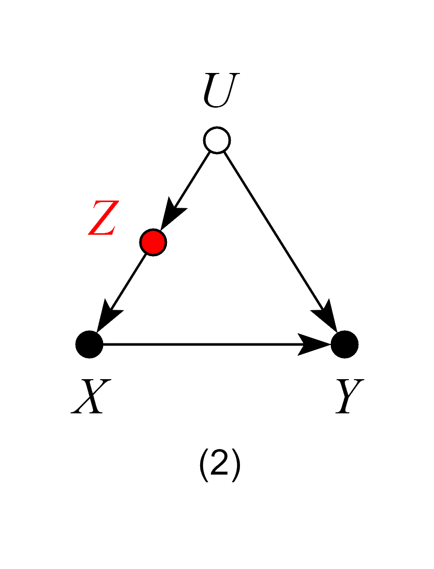
In the following set of models, the target of the analysis is the average causal effect (ACE) of a treatment X on an outcome Y, which stands for the expected increase of Y per unit of a controlled increase in X. Observed variables will be designated by black dots and unobserved variables by white empty circles. Variable Z (highlighted in red) will represent the variable whose inclusion in the regression is to be decided, with “good control” standing for bias reduction, “bad control” standing for bias increase and “netral control” when the addition of Z does not increase nor reduce bias. For this last case, we will also make a brief remark about how Z could affect the precision of the ACE estimate.
Models
Models 1, 2 and 3 – Good Controls
In model 1, Z stands for a common cause of both X and Y. Once we control for Z, we block the back-door path from X to Y, producing an unbiased estimate of the ACE.
In models 2 and 3, Z is not a common cause of both X and Y, and therefore, not a traditional “confounder” as in model 1. Nevertheless, controlling for Z blocks the back-door path from X to Y due to the unobserved confounder U, and again, produces an unbiased estimate of the ACE.
Models 4, 5 and 6 – Good Controls
When thinking about possible threats of confounding, one needs to keep in mind that common causes of X and any mediator (between X and Y) also confound the effect of X on Y. Therefore, models 4, 5 and 6 are analogous to models 1, 2 and 3 — controlling for Z blocks the backdoor path from X to Y and produces an unbiased estimate of the ACE.
Model 7 – Bad Control
We now encounter our first “bad control”. Here Z is correlated with the treatment and the outcome and it is also a “pre-treatment” variable. Traditional econometrics textbooks would deem Z a “good control”. The backdoor criterion, however, reveals that Z is a “bad control”. Controlling for Z will induce bias by opening the backdoor path X ← U1→ Z← U2→Y, thus spoiling a previously unbiased estimate of the ACE.
Model 8 – Neutral Control (possibly good for precision)
Here Z is not a confounder nor does it block any backdoor paths. Likewise, controlling for Z does not open any backdoor paths from X to Y. Thus, in terms of bias, Z is a “neutral control”. Analysis shows, however, that controlling for Z reduces the variation of the outcomevariable Y, and helps improve the precision of the ACE estimate in finite samples.
Model 9 – Neutral control (possibly bad for precision)
Similar to the previous case, here Z is “neutral” in terms of bias reduction. However, controlling for Z will reduce the variation of treatment variable X and so may hurt the precision of the estimate of the ACE in finite samples.
Model 10 – Bad control
We now encounter our second “pre-treatment” “bad control”, due to a phenomenon called “bias amplification” (read more here). Naive control for Z in this model will not only fail to deconfound the effect of X on Y, but, in linear models, will amplify any existing bias.
Models 11 and 12 – Bad Controls
If our target quantity is the ACE, we want to leave all channels through which the causal effect flows “untouched”.
In Model 11, Z is a mediator of the causal effect of X on Y. Controlling for Z will block the very effect we want to estimate, thus biasing our estimates.
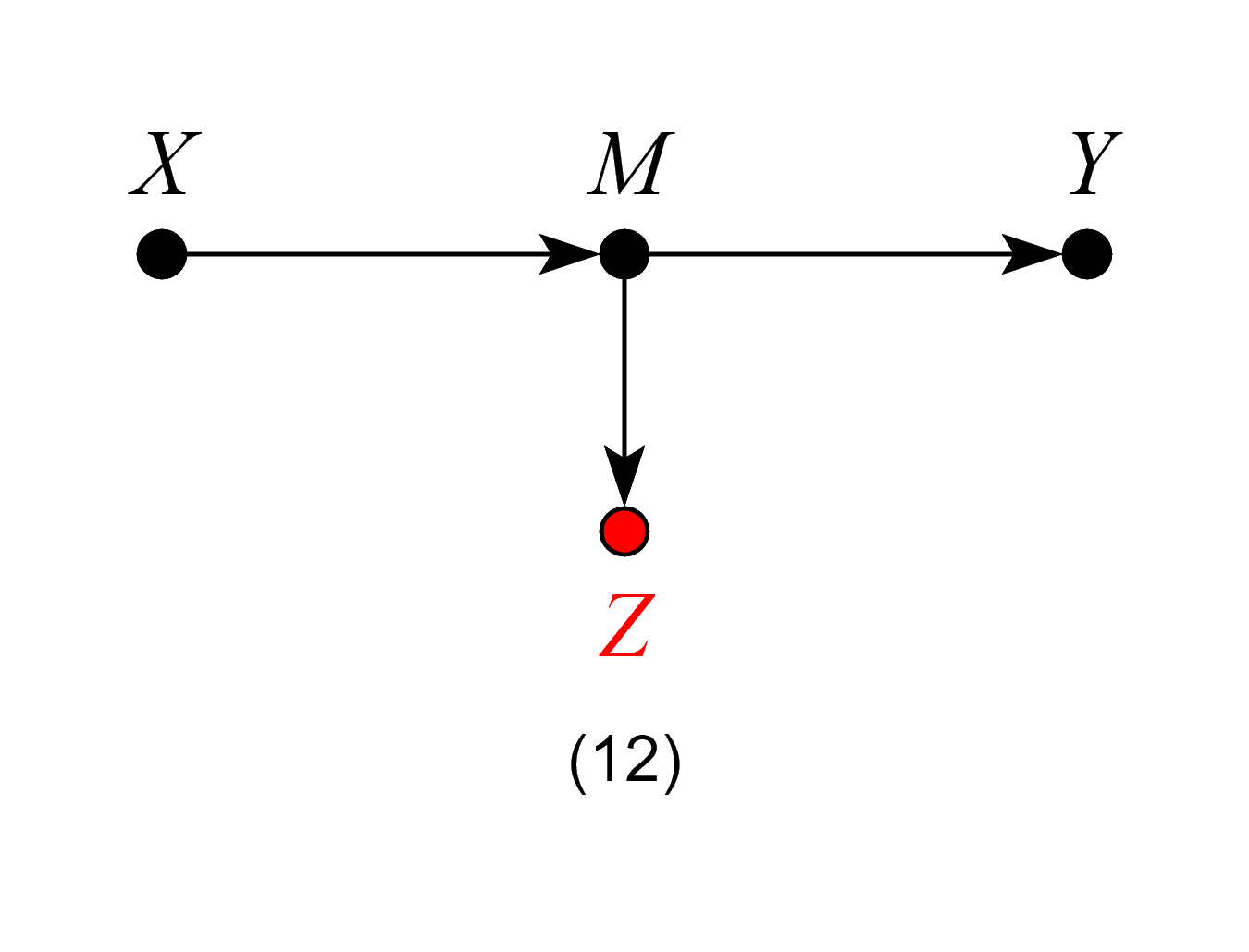
In Model 12, although Z is not itself a mediator of the causal effect of X on Y, controlling for Z is equivalent to partially controlling for the mediator M, and will thus bias our estimates.
Models 11 and 12 violate the backdoor criterion, which excludes controls that are descendants of the treatment along paths to the outcome.
Model 13 – Neutral control (possibly good for precision)
At first look, model 13 might seem similar to model 12, and one may think that adjusting for Z would bias the effect estimate, by restricting variations of the mediator M. However, the key difference here is that Z is a cause, not an effect, of the mediator (and, consequently, also a cause of Y). Thus, model 13 is analogous to model 8, and so controlling for Z will be neutral in terms of bias and may increase precision of the ACE estimate in finite samples.
Model 14 – Neutral controls (possibly helpful in the case of selection bias)
Contrary to econometrics folklore, not all “post-treatment” variables are inherently bad controls. In models 14 and 15 controlling for Z does not open any confounding paths between X and Y. Thus, Z is neutral in terms of bias. However, controlling for Z does reduce the variation of the treatment variable X and so may hurt the precision of the ACE estimate in finite samples. Additionally, in model 15, suppose one has only samples with W = 1 recorded (a case of selection bias). In this case, controlling for Z can help obtaining the W-specific effect of X on Y, by blocking the colliding path due to W.
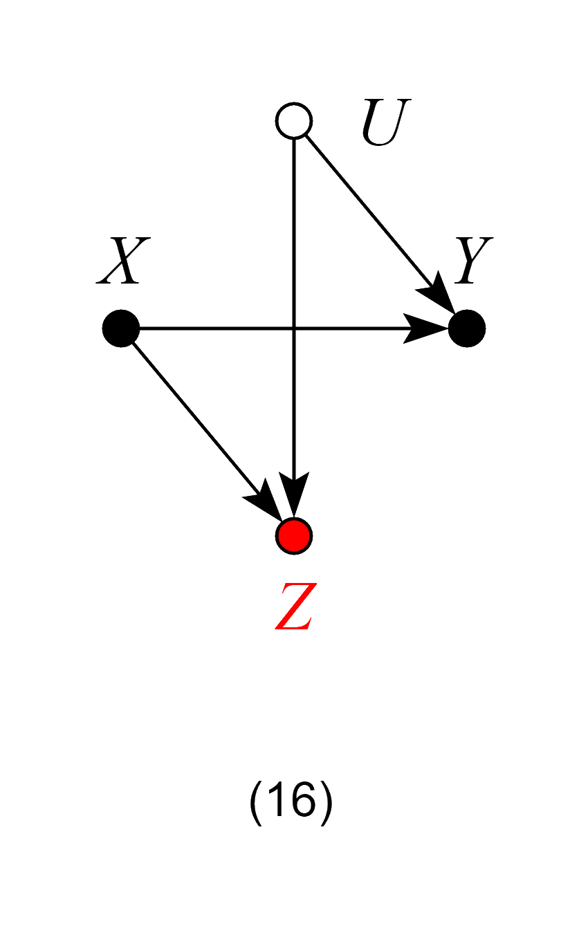
Model 16 – Bad control
Contrary to Models 14 and 15, here controlling for Z is no longer harmless, since it opens the backdoor path X → Z ← U → Y and so biases the ACE.
Model 17 – Bad Control
Here, Z is not a mediator, and one might surmise that, as in Model 14, controlling for Z is harmless. However, controlling for the effects of the outcome Y will induce bias in the estimate of the ACE, making Z a “bad control”. A visual explanation of this phenomenon using “virtual colliders” can be found here.
Model 17 is usually known as a “case-control bias” or “selection bias”. Finally, although controlling for Z will generally bias numerical estimates of the ACE, it does have an exception when X has no causal effect on Y. In this scenario, X is still d-separated from Y even after conditioning on Z. Thus, adjusting for Z is valid for testing whether the effect of X on Y is zero.
Andrew Gelman and his blog readers followed-up with the previous discussion (link here) on his methods to address issues about causal inference and transportability of causal effects based on his “hierarchical modeling” framework, and I just posted my answer.
In the past week, I have been engaged in a discussion with Andrew Gelman and his blog readers regarding causal inference, selection bias, confounding, and generalizability. I was trying to understand how his method which he calls “hierarchical modelling” would handle these issues and what guarantees it provides. Unfortunately, I could not reach an understanding of Gelman’s method (probably because no examples were provided).
If anyone understands how “hierarchical modeling” can solve a simple toy problem (e.g., M-bias, control of confounding, mediation, generalizability), please share with us.
I have tried to read Judea and Ilya's paper on effect of treatment on the treated which sound much more general than anything else I have read on the subject before. Unfortunately I was unable to follow their proof and could not find an instance where the ETT effect is identifiable. The only instance where I new that ETT was identifiable is with an instrumental variable under certain restrictions, instead I imagine that identifiability here means without restrictions other than those encoded in the DAG.The most clear treatment of the subject I new until now is in a paper by Hernan and Robins in Epidemiology 2006; and I do not understand why the discussion on Forcina's paper by Robins, Vander Weele and RIchardson is so popular.
The parameter identification method described in Section 5.3.1 rests on two criteria: (1) The single door criterion of Theorem 5.3.1, and the back-door criterion of Theorem 5.3.2. This method may require appreciable bookkeeping in combining results from various segments of the graph. Is there a single graphical criterion of identification that unifies the two Theorems and thus avoids much of the bookkeeping involved?
 In chapter 19, Boole first showed the following: