Causal Analysis in Theory and Practice

May 31, 2020

What Statisticians Want to Know about Causal Inference and The Book of Why

Filed under: Causal Effect,DAGs,Discussion,Economics,Epidemiology,Opinion — Judea Pearl @ 4:09 pm

I was privileged to be interviewed recently by David Hand, Professor of Statistics at Imperial College, London, and a former President of the Royal Statistical Society. I would like to share this interview with readers of this blog since many of the questions raised by David keep coming up in my conversations with statisticians and machine learning researchers, both privately and on Twitter.

For me, David represents mainstream statistics and, the reason I find his perspective so valuable is that he does not have a stake in causality and its various formulations. Like most mainstream statisticians, he is simply curious to understand what the big fuss is all about and how to communicate differences among various approaches without taking sides.

So, I’ll let David start, and I hope you find it useful.

Judea Pearl Interview by David Hand

There are some areas of statistics which seem to attract controversy and disagreement, and causal modelling is certainly one of them. In an attempt to understand what all the fuss is about, I asked Judea Pearl about these differences in perspective. Pearl is a world leader in the scientific understanding of causality. He is a recipient of the AMC Turing Award (computing’s “Nobel Prize”), for “fundamental contributions to artificial intelligence through the development of a calculus for probabilistic and causal reasoning”, the David E. Rumelhart Prize for Contributions to the Theoretical Foundations of Human Cognition, and is a Fellow of the American Statistical Association.

QUESTION 1:

I am aware that causal modelling is a hotly contested topic, and that there are alternatives to your perspective – the work of statisticians Don Rubin and Phil Dawid spring to mind, for example. Words like counterfactual, Popperian falsifiability, potential outcomes, appear. I’d like to understand the key differences between the various perspectives, so can you tell me what are the main grounds on which they disagree?

ANSWER 1:

You might be surprised to hear that, despite what seems to be hotly contested debates, there are very few philosophical differences among the various “approaches.” And I put “approaches” in quotes because the differences are more among historical traditions, or “frameworks” than among scientific principles. If we compare, for example, Rubin’s potential outcome with my framework, named “Structural Causal Models” (SCM), we find that the two are logically equivalent; a theorem in one is a theorem in the other and an assumption in one can be written as an assumption in the other. This means that, starting with the same set of assumptions, every solution obtained in one can also be obtained in the other.

But logical equivalence does not means “modeling equivalence” when we consider issues such as transparency, credibility or tractability. The equations for straight lines in polar coordinates are equivalent to those in Cartesian coordinates yet are hardly manageable when it comes to calculating areas of squares or triangles.

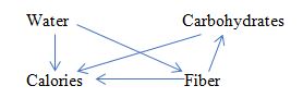
In SCM, assumptions are articulated in the form of equations among measured variables, each asserting how one variable responds to changes in another. Graphical models are simple abstractions of those equations and, remarkably, are sufficient for answering many causal questions when applied to non-experimental data. An arrow X—>Y in a graphical model represents the capacity to respond to such changes. All causal relationships are derived mechanically from those qualitative primitives, demanding no further judgment of the modeller.

In Rubin’s framework, assumptions are expressed as conditional independencies among counterfactual variables, also known as “ignorability conditions.” The mental task of ascertaining the plausibility of such assumptions is beyond anyone’s capacity, which makes it extremely hard for researchers to articulate or to verify. For example, the task of deciding which measurements to include in the analysis (or in the propensity score) is intractable in the language of conditional ignorability. Judging whether the assumptions are compatible with the available data, is another task that is trivial in graphical models and insurmountable in the potential outcome framework.

Conceptually, the differences can be summarized thus: The graphical approach goes where scientific knowledge resides, while Rubin’s approach goes where statistical routines need to be justified. The difference shines through when simple problems are solved side by side in both approaches, as in my book Causality (2009). The main reason differences between approaches are still debated in the literature is that most statisticians are watching these debates as outsiders, instead of trying out simple examples from beginning to end. Take for example Simpson’s paradox, a puzzle that has intrigued a century of statisticians and philosophers. It is still as vexing to most statisticians today as it was to Pearson in 1889, and the task of deciding which data to consult, the aggregated or the disaggregated is still avoided by all statistics textbooks.

To summarize, causal modeling, a topic that should be of prime interest to all statisticians, is still perceived to be a “hotly contested topic”, rather than the main frontier of statistical research. The emphasis on “differences between the various perspectives” prevents statisticians from seeing the exciting new capabilities that now avail themselves, and which “enable us to answer questions that we have always wanted but were afraid to ask.” It is hard to tell whether fears of those “differences” prevent statisticians from seeing the excitement, or the other way around, and cultural inhibitions prevent statisticians from appreciating the excitement, and drive them to discuss “differences” instead.

QUESTION 2:

There are different schools of statistics, but I think that most modern pragmatic applied statisticians are rather eclectic, and will choose a method which has the best capability to answer their particular questions. Does the same apply to approaches to causal modelling? That is, do the different perspectives have strengths and weaknesses, and should we be flexible in our choice of approach?

ANSWER 2:

These strengths and weaknesses are seen clearly in the SCM framework, which unifies several approaches and provides a flexible way of leveraging the merits of each. In particular, SCM combines graphical models and potential outcome logic. The graphs are used to encode what we know (i.e., the assumptions we are willing to defend) and the logic is used to encode what we wish to know, that is, the research question of interest. Simple mathematical tools can then combine these two with data and produce consistent estimates.

The availability of these unifying tools now calls on statisticians to become actively involved in causal analysis, rather than attempting to judge approaches from a distance. The choice of approach will become obvious once research questions are asked and the stage is set to articulate subject matter information that is necessary in answering those questions.

QUESTION 3:

To a very great extent the modern big data revolution has been driven by so-called “databased” models and algorithms, where understanding is not necessarily relevant or even helpful, and where there is often no underlying theory about how the variables are related. Rather, the aim is simply to use data to construct a model or algorithm which will predict an outcome from input variables (deep learning neural networks being an illustration). But this approach is intrinsically fragile, relying on an assumption that the data properly represent the population of interest. Causal modelling seems to me to be at the opposite end of the spectrum: it is intrinsically “theory-based”, because it has to begin with a causal model. In your approach, described in an accessible way in your recent book The Book of Why, such models are nicely summarised by your arrow charts. But don’t theory-based models have the complementary risk that they rely heavily on the accuracy of the model? As you say on page 160 of The Book of Why, “provided the model is correct”.

ANSWER 3:

When the tasks are purely predictive, model-based methods are indeed not immediately necessary and deep neural networks perform surprisingly well. This is level-1 (associational) in the Ladder of Causation described in The Book of Why. In tasks involving interventions, however (level-2 of the Ladder), model-based methods become a necessity. There is no way to predict the effect of policy interventions (or treatments) unless we are in possession of either causal assumptions or controlled randomized experiments employing identical interventions. In such tasks, and absent controlled experiments, reliance on the accuracy of the model is inevitable, and the best we can do is to make the model transparent, so that its accuracy can be (1) tested for compatibility with data and/or (2) judged by experts as well as policy makers and/or (3) subjected to sensitivity analysis.

A major reason why statisticians are reluctant to state and rely on untestable modeling assumptions stems from lack of training in managing such assumptions, however plausible. Even stating such unassailable assumptions as “symptoms do not cause diseases” or “drugs do not change patient’s sex” require a vocabulary that is not familiar to the great majority of living statisticians. Things become worse in the potential outcome framework where such assumptions resist intuitive interpretation, let alone judgment of plausibility. It is important at this point to go back and qualify my assertion that causal models are not necessary for purely predictive tasks. Many tasks that, at first glance appear to be predictive, turn out to require causal analysis. A simple example is the problem of external validity or inference across populations. Differences among populations are very similar to differences induced by interventions, hence methods of transporting information from one population to another can leverage all the tools developed for predicting effects of interventions. A similar transfer applies to missing data analysis, traditionally considered a statistical problem. Not so. It is inherently a causal problem since modeling the reason for missingness is crucial for deciding how we can recover from missing data. Indeed modern methods of missing data analysis, employing causal diagrams are able to recover statistical and causal relationships that purely statistical methods have failed to recover.

QUESTION 4:

In a related vein, the “backdoor” and “frontdoor” adjustments and criteria described in the book are very elegant ways of extracting causal information from arrow diagrams. They permit causal information to be obtained from observational data. Provided that is, the arrow diagram accurately represents the relationships between all the relevant variables. So doesn’t valid application of this elegant calculus depends critically on the accuracy of the base diagram?

ANSWER 4:

Of course. But as we have agreed above, EVERY exercise in causal inference “depends critically on the accuracy” of the theoretical assumptions we make. Our choice is whether to make these assumptions transparent, namely, in a form that allows us to scrutinize their veracity, or bury those assumptions in cryptic notation that prevents scrutiny.

In a similar vein, I must modify your opening statement, which described the “backdoor” and “frontdoor” criteria as “elegant ways of extracting causal information from arrow diagrams.” A more accurate description would be “…extracting causal information from rudimentary scientific knowledge.” The diagrammatic description of these criteria enhances, rather than restricts their range of applicability. What these criteria in fact do is extract quantitative causal information from conceptual understanding of the world; arrow diagrams simply represent the extent to which one has or does not have such understanding. Avoiding graphs conceals what knowledge one has, as well as what doubts one entertains.

QUESTION 5:

You say, in The Book of Why (p5-6) that the development of statistics led it to focus “exclusively on how to summarise data, not on how to interpret it.” It’s certainly true that when the Royal Statistical Society was established it focused on “procuring, arranging, and publishing ‘Facts calculated to illustrate the Condition and Prospects of Society’,” and said that “the first and most essential rule of its conduct [will be] to exclude carefully all Opinions from its transactions and publications.” But that was in the 1830s, and things have moved on since then. Indeed, to take one example, clinical trials were developed in the first half of the Twentieth Century and have a history stretching back even further. The discipline might have been slow to get off the ground in tackling causal matters, but surely things have changed and a very great deal of modern statistics is directly concerned with causal matters – think of risk factors in epidemiology or manipulation in experiments, for example. So aren’t you being a little unfair to the modern discipline?

ANSWER 5:

Ronald Fisher’s manifesto, in which he pronounced that “the object of statistical methods is the reduction of data” was published in 1922, not in the 19th century (Fisher 1922). Data produced in clinical trials have been the only data that statisticians recognize as legitimate carriers of causal information, and our book devotes a whole chapter to this development. With the exception of this singularity, however, the bulk of mainstream statistics has been glaringly disinterested in causal matters. And I base this observation on three faithful indicators: statistics textbooks, curricula at major statistics departments, and published texts of Presidential Addresses in the past two decades. None of these sources can convince us that causality is central to statistics.

Take any book on the history of statistics, and check if it considers causal analysis to be of primary concern to the leading players in 20th century statistics. For example, Stigler’s The Seven Pillars of Statistical Wisdom (2016) barely makes a passing remark to two (hardly known) publications in causal analysis.

I am glad you mentioned epidemiologists’ analysis of risk factors as an example of modern interest in causal questions. Unfortunately, epidemiology is not representative of modern statistics. In fact epidemiology is the one field where causal diagrams have become a second language, contrary to mainstream statistics, where causal diagrams are still a taboo. (e.g., Efron and Hastie 2016; Gelman and Hill, 2007; Imbens and Rubin 2015; Witte and Witte, 2017).

When an academic colleague asks me “Aren’t you being a little unfair to our discipline, considering the work of so and so?”, my answer is “Must we speculate on what ‘so and so’ did? Can we discuss the causal question that YOU have addressed in class in the past year?” The conversation immediately turns realistic.

QUESTION 6:

Isn’t the notion of intervening through randomisation still the gold standard for establishing causality?

ANSWER 6:

It is. Although in practice, the hegemony of randomized trial is being contested by alternatives. Randomized trials suffer from incurable problems such as selection bias (recruited subject are rarely representative of the target population) and lack of transportability (results are not applicable when populations change). The new calculus of causation helps us overcome these problems, thus achieving greater over all credibility; after all, observational studies are conducted at the natural habitat of the target population.

QUESTION 7:

What would you say are the three most important ideas in your approach? And what, in particular, would you like readers of The Book of Why to take away from the book.

ANSWER 7:

The three most important ideas in the book are: (1) Causal analysis is easy, but requires causal assumptions (or experiments) and those assumptions require a new mathematical notation, and a new calculus. (2) The Ladder of Causation, consisting of (i) association (ii) interventions and (iii) counterfactuals, is the Rosetta Stone of causal analysis. To answer a question at layer (x) we must have assumptions at level (x) or higher. (3) Counterfactuals emerge organically from basic scientific knowledge and, when represented in graphs, yield transparency, testability and a powerful calculus of cause and effect. I must add a fourth take away: (4) To appreciate what modern causal analysis can do for you, solve one toy problem from beginning to end; it would tell you more about statistics and causality than dozens of scholarly articles laboring to overview statistics and causality.

REFERENCES

Efron, B. and Hastie, T., Computer Age Statistical Inference: Algorithms, Evidence, and Data Science, New York, NY: Cambridge University Press, 2016.

Fisher, R., “On the mathematical foundations of theoretical statistics,” Philosophical Transactions of the Royal Society of London, Series A 222, 311, 1922.

Gelman, A. and Hill, J., Data Analysis Using Regression and Multilevel/Hierarchical Models, New York: Cambridge University Press, 2007.

Imbens, G.W. and Rubin, D.B., Causal Inference for Statistics, Social, and Biomedical Sciences: An Introduction, Cambridge, MA: Cambridge University Press, 2015.

Witte, R.S. and Witte, J.S., Statistics, 11th edition, Hoboken, NJ: John Wiley & Sons, Inc. 2017.

Comments (0)

June 15, 2018

A Statistician’s Re-Reaction to The Book of Why

Filed under: Book (J Pearl),Discussion,Simpson's Paradox — Judea Pearl @ 2:29 am

Responding to my June 11 comment, Kevin Gray posted a reply on kdnuggets.com in which he doubted the possibility that the Causal Revolution has solved problems that generations of statisticians and philosophers have labored over and could not solve. Below is my reply to Kevin’s Re-Reaction, which I have also submitted to kdhuggets.com:

Dear Kevin,
I am not suggesting that you are only superficially acquainted with my works. You actually show much greater acquaintance than most statisticians in my department, and I am extremely appreciative that you are taking the time to comment on The Book of Why. You are showing me what other readers with your perspective would think about the Book, and what they would find unsubstantiated or difficult to swallow. So let us go straight to these two points (i.e., unsubstantiated and difficult to swallow) and give them an in-depth examination.

You say that I have provided no evidence for my claim: “Even today, only a small percentage of practicing statisticians can solve any of the causal toy problems presented in the Book of Why.” I believe that I did provide such evidence, in each of the Book’s chapters, and that the claim is valid once we agree on what is meant by “solve.”

Let us take the first example that you bring, Simpson’s paradox, which is treated in Chapter 6 of the Book, and which is familiar  to every red-blooded statistician. I characterized the paradox in these words: “It has been bothering statisticians for more than sixty years – and it remains vexing to this very day” (p. 201). This was, as you rightly noticed, a polite way of saying: “Even today, the vast majority of statisticians cannot solve Simpson’s paradox,” a fact which I strongly believe to be true.

You find this statement hard to swallow, because: “generations of researchers and statisticians have been trained to look out for it [Simpson’s Paradox]” an observation that seems to contradict my claim. But I beg you to note that “trained to look out for it” does not make the researchers capable of “solving it,” namely capable of deciding what to do when the paradox shows up in the data.

This distinction appears vividly in the debate that took place in 2014 on the pages of The American Statistician, which you and I cite.  However, whereas you see the disagreements in that debate as evidence that statisticians have several ways of resolving Simpson’s paradox, I see it as evidence that they did not even come close. In other words, none of the other participants presented a method for deciding whether the aggregated data or the segregated data give the correct answer to the question: “Is the treatment helpful or harmful?”

Please pay special attention to the article by Keli Liu and Xiao-Li Meng, both are from Harvard’s department of statistics (Xiao-Li is a senior professor and a Dean), so they cannot be accused of misrepresenting the state of statistical knowledge in 2014. Please read their paper carefully and judge for yourself whether it would help you decide whether treatment is helpful or not, in any of the examples presented in the debate.

It would not!! And how do I know? I am listening to their conclusions:

  1. They disavow any connection to causality (p.18), and
  2. They end up with the wrong conclusion. Quoting: “less conditioning is most likely to lead to serious bias when Simpson’s Paradox appears.” (p.17) Simpson himself brings an example where conditioning leads to more bias, not less.

I dont blame Liu and Meng for erring on this point, it is not entirely their fault (Rosenbaum and Rubin made the same error). The correct solution to Simpson’s dilemma rests on the back-door criterion, which is almost impossible to articulate without the aid of DAGs. And DAGs, as you are probably aware, are forbidden from entering a 5 mile no-fly zone around Harvard [North side, where the statistics department is located].

So, here we are. Most statisticians believe that everyone knows how to “watch for” Simpson’s paradox, and those who seek an answer to: “Should we treat or not?” realize that “watching” is far from “solving.” Moreover, the also realize that there is no solution without stepping outside the comfort zone of statistical analysis and entering the forbidden city of causation and graphical models.

One thing I do agree with you — your warning about the implausibility of the Causal Revolution. Quoting: “to this day, philosophers disagree about what causation is, thus to suggest he has found the answer to it is not plausible”.  It is truly not plausible that someone, especially a semi-outsider, has found a Silver Bullet. It is hard to swallow. That is why I am so excited about the Causal Revolution and that is why I wrote the book. The Book does not offer a Silver Bullet to every causal problem in existence, but it offers a solution to a class of problems that centuries of statisticians and Philosophers tried and could not crack. It is implausible, I agree, but it happened. It happened not because I am smarter but because I took Sewall Wright’s idea seriously and milked it to its logical conclusions as much as I could.

It took quite a risk on my part to sound pretentious and call this development a Causal Revolution. I thought it was necessary. Now I am asking you to take a few minutes and judge for yourself whether the evidence does not justify such a risky characterization.

It would be nice if we could alert practicing statisticians, deeply invested in the language of statistics to the possibility that paradigm shifts can occur even in the 21st century, and that centuries of unproductive debates do not make such shifts impossible.

You were right to express doubt and disbelief in the need for a paradigm shift, as would any responsible scientist in your place. The next step is to let the community explore:

  1. How many statisticians can actually answer Simpson’s question, and
  2. How to make that number reach 90%.

I believe The Book of Why has already doubled that number, which is some progress. It is in fact something that I was not able to do in the past thirty years through laborious discussions with the leading statisticians of our time.

It is some progress, let’s continue,
Judea

Comments (4)

January 24, 2018

Can DAGs Do the Un-doable?

Filed under: DAGs,Discussion — Judea Pearl @ 2:32 am

The following question was sent to us by Igor Mandel:

Separation of variables with zero causal coefficients from others
Here is a problem. Imagine, we have a researcher who has some understanding of the particular problem, and this understanding is partly or completely wrong. Can DAG or other (if any) causality theory convincingly establish this fact (that she is wrong)?

To be more specific, let’s consider a simple example with kind of undisputable causal variables (described in details in https://papers.ssrn.com/sol3/papers.cfm?abstract_id=2984045 ). One wants to estimate, how different food’s ingredients affect the energy (in calories) containing in different types of food. She takes many samples and measures different things. But she doesn’t know about existence of the fats and proteins – yet she knows, that there are carbohydrates, water and fiber. She builds a respective DAG, how she feels it should be:

From our (i.e. educated people of 21st century) standpoint the arrows from Fiber and Water to Calories have zero coefficients. But since data bear significant correlations between Calories, Water and Fiber – any regression estimates would show non-zero values for these coefficients. Is there way to say, that these non-zero values are wrong, not just quantitatively, but kind of qualitatively?
Even brighter example of what is often called “spurious correlation”. It was “statistically proven” almost 20 years ago, that storks deliver babies ( http://robertmatthews.org/wp-content/uploads/2016/03/RM-storks-paper.pdf ) – while many women still believe they do not. How to reconvince those statistically ignorant women? Or – how to strengthen their naïve, but statistically not confirmed beliefs, just looking at the data and not asking them for some babies related details? What kind of DAG may help?

My Response
This question, in a variety of settings, has been asked by readers of this blog since the beginning of the Causal Revolution. The idea that new tools are now available that can handle causal problems free of statistical dogmas has encouraged thousands of researchers to ask: Can you do this, or can you do that? The answers to such questions are often trivial, and can be obtained directly from the logic of causal inference, without the details of the question. I am not surprised however that such questions surface again, in 2018, since the foundations of causal inference are rarely emphasized in the technical literature, so they tend to be forgotten.

I will answer Igor’s question as a student of modern logic of causation.

1. Can a DAG distinguish variables with zero causal effects (on Y) from those having non-zero effects.

Of course not, no method in the world can do that without further assumption. Here is why:
The question above concerns causal relations. We know from first principle that no causal query can be answered from data alone, without causal information that lies outside the data.
QED
[It does not matter if your query is quantitative or qualitative, if you address it to a story or to a graph. Every causal query needs causal assumptions. No causes in – no causes out (N. Cartwright)]

2. Can DAG-based methods do anything more than just quit with failure?

Of course they can.

2.1 First notice that the distinction between having or not having causal effect is a property of nature, (or the data generating process), not of the model that you postulate. We can therefore ignore the diagram that Igor describes above. Now, in addition to quitting for lack of information, DAG-based methods would tell you: “If you can give me some causal information, however qualitative, I will tell you if it is sufficient or not for answering your query.” I hope readers would agree with me that this kind of an answer, though weaker than the one expected by the naïve inquirer, is much more informative than just quitting in despair.

2.2 Note also that postulating a whimsical model like the one described by Igor above has no bearing on the answer. To do anything useful in causal inference we need to start with a model of reality, not with a model drawn by a confused researcher, for whom an arrow is nothing more than “data bears significant correlation” or “regression estimates show non-zero values.”

2.3 Once you start with a postulated model of reality, DAG-based methods can be very helpful. For example, they can take your postulated model and determine which of the arrows in the model should have a zero coefficient attached to it, which should have a non-zero coefficient attached to it, and which would remain undecided till the end of time.

2.4 Moreover, assume reality is governed by model M1 and you postulate model M2, different from M1. DAG-based methods can tell you which causal query you will answer correctly and which you will
answer incorrectly. (see section 4.3 of http://ftp.cs.ucla.edu/pub/stat_ser/r459-reprint-errata.pdf ). This is nice, because it offers us a kind of sensitivity analysis: how far should reality be from your assumed model before you will start making mistakes?

2.5 Finally, DAG-based methods identify for us the testable implication of our model, so that we can test models for compatibility with data.

I am glad Igor raised the question that he did. There is a tendency to forget fundamentals, and it is healthy to rehearse them periodically.

– Judea

Comments (13)

August 2, 2017

2017 Mid-Summer Update

Filed under: Counterfactual,Discussion,Epidemiology — Judea Pearl @ 12:55 am

Dear friends in causality research,

Welcome to the 2017 Mid-summer greeting from the Ucla Causality Blog.

This greeting discusses the following topics:

1. “The Eight Pillars of Causal Wisdom” and the WCE 2017 Virtual Conference Website.
2. A discussion panel: “Advances in Deep Neural Networks”,
3. Comments on “The Tale Wagged by the DAG”,
4. A new book: “The book of Why”,
5. A new paper: Disjunctive Counterfactuals,
6. Causality in Education Award,
7. News on “Causal Inference: A  Primer”

1. “The Eight Pillars of Causal Wisdom”


The tenth annual West Coast Experiments Conference was held at UCLA on April 24-25, 2017, preceded by a training workshop  on April 23.

You will be pleased to know that the WCE 2017 Virtual Conference Website is now available here:
http://spp.ucr.edu/wce2017/
It provides videos of the talks as well as some of the papers and presentations.

The conference brought together scholars and graduate students in economics, political science and other social sciences who share an interest in causal analysis. Speakers included:

1. Angus Deaton, on Understanding and misunderstanding randomized controlled trials.
2. Chris Auld, on the on-going confusion between regression vs. structural equations in the econometric literature.
3. Clark Glymour, on Explanatory Research vs Confirmatory Research.
4. Elias Barenboim, on the solution to the External Validity problem.
5. Adam Glynn, on Front-door approaches to causal inference.
6. Karthika Mohan, on Missing Data from a causal modeling perspective.
7. Judea Pearl, on “The Eight Pillars of Causal Wisdom.”
8. Adnan Darwiche, on Model-based vs. Model-Blind Approaches to Artificial Intelligence.
9. Niall Cardin, Causal inference for machine learning.
10. Karim Chalak, Measurement Error without Exclusion.
11. Ed Leamer, “Causality Complexities Example: Supply and Demand.
12. Rosa Matzkin, “Identification is simultaneous equation.
13 Rodrigo Pinto, Randomized Biased-controlled Trials.

The video of my lecture “The Eight Pillars of Causal Wisdom” can be watched here:
https://www.youtube.com/watch?v=8nHVUFqI0zk
A transcript of the talk can be found here:
http://spp.ucr.edu/wce2017/Papers/eight_pillars_of.pdf

2. “Advances in Deep Neural Networks”


As part of the its celebration of the 50 years of the Turing Award, the ACM has organized several discussion sessions on selected topics in computer science. I participated in a panel discussion on
“Advances in Deep Neural Networks”, which gave me an opportunity to share thoughts on whether learning methods based solely on data fitting can ever achieve a human-level intelligence. The discussion video can be viewed here:
https://www.youtube.com/watch?v=mFYM9j8bGtg
A position paper that defends these thoughts is available here:
web.cs.ucla.edu/~kaoru/theoretical-impediments.pdf

3. The Tale Wagged by the DAG


An article by this title, authored by Nancy Krieger and George Davey Smith has appeared in the International Journal of Epidemiology, IJE 2016 45(6) 1787-1808.
https://academic.oup.com/ije/issue/45/6#250304-2617148
It is part of a special IJE issue on causal analysis which, for the reasons outlined below, should be of interest to readers of this blog.

As the title tell-tales us, the authors are unhappy with the direction that modern epidemiology has taken, which is too wedded to a two-language framework:
(1) Graphical models (DAGs) — to express what we know, and
(2) Counterfactuals (or potential outcomes) — to express what we wish to know.

The specific reasons for the authors unhappiness are still puzzling to me, because the article does not demonstrate concrete alternatives to current methodologies. I can only speculate however that it is the dazzling speed with which epidemiology has modernized its tools that lies behind the authors discomfort. If so, it would be safe for us to assume that the discomfort will subside as soon as researchers gain greater familiarity with the capabilities and flexibility of these new tools.  I nevertheless recommend that the article, and the entire special issue of IJE be studied by our readers, because they reflect an interesting soul-searching attempt by a forward-looking discipline to assess its progress in the wake of a profound paradigm shift.

Epidemiology, as I have written on several occasions, has been a pioneer in accepting the DAG-counterfactuals symbiosis as a ruling paradigm — way ahead of mainstream statistics and its other satellites. (The social sciences, for example, are almost there, with the exception of the model-blind branch of econometrics. See Feb. 22 2017 posting)

In examining the specific limitations that Krieger and Davey Smith perceive in DAGs, readers will be amused to note that these limitations coincide precisely with the strengths for which DAGs are praised.

For example, the article complains that DAGs provide no information about variables that investigators chose not to include in the model.  In their words: “the DAG does not provide a comprehensive picture. For example, it does not include paternal factors, ethnicity, respiratory infections or socioeconomic position…” (taken from the Editorial introduction). I have never considered this to be a limitation of DAGs or of any other scientific modelling. Quite the contrary. It would be a disaster if models were permitted to provide information unintended by the modeller. Instead, I have learned to admire the ease with which DAGs enable researchers to incorporate knowledge about new variables, or new mechanisms, which the modeller wishes
to embrace.

Model misspecification, after all,  is a problem that plagues every  exercise in causal inference, no matter what framework one chooses to adapt. It can only be cured by careful model-building
strategies, and by enhancing the modeller’s knowledge. Yet, when it comes to minimizing misspecification errors, DAGS have no match. The transparency with which DAGs display the causal assumptions in the model, and the ease with which the DAG identifies the testable implications of those assumptions are incomparable; these facilitate speedy model diagnosis and repair with no match in sight.

Or, to take another example, the authors call repeatedly for an ostensibly unavailable methodology which they label “causal triangulation” (it appears 19 times in the article). In their words: “In our field, involving dynamic populations of people in dynamic societies and ecosystems, methodical triangulation of diverse types of evidence from diverse types of study settings and involving diverse populations is essential.”  Ironically, however, the task of treating “diverse type of evidence from diverse populations” has been accomplished quite successfully in the dag-counterfactual framework. See, for example the formal and complete results of (Bareinbaum and Pearl, 2016, http://ftp.cs.ucla.edu/pub/stat_ser/r450-reprint.pdf) which have emerged from DAG-based perspective and invoke the do-calculus. (See also  http://ftp.cs.ucla.edu/pub/stat_ser/r400.pdf) It is inconceivable for me to imagine anyone pooling data from two different designs (say
experimental and observational) without resorting to DAGs or (equivalently) potential outcomes, I am open to learn.

Another conceptual paradigm which the authors hope would liberate us from the tyranny of DAGs and counterfactuals is Lipton’s (2004) romantic aspiration for “Inference to the Best Explanation.” It is a compelling, century old mantra, going back at least to Charles Pierce theory of abduction (Pragmatism and Pragmaticism, 1870) which, unfortunately, has never operationalized its key terms: “explanation,” “Best” and “inference to”.  Again, I know of only one framework in which this aspiration has been explicated with sufficient precision to produce tangible results — it is the structural framework of DAGs and counterfactuals. See, for example, Causes of Effects and Effects of Causes”
http://ftp.cs.ucla.edu/pub/stat_ser/r431-reprint.pdf
and Halpern and Pearl (2005) “Causes and explanations: A structural-model approach”
http://ftp.cs.ucla.edu/pub/stat_ser/r266-part1.pdf

In summary, what Krieger and Davey Smith aspire to achieve by abandoning the structural framework has already been accomplished with the help and grace of that very framework.
More generally, what we learn from these examples is that the DAG-counterfactual symbiosis is far from being a narrow “ONE approach to causal inference” which ” may potentially lead to spurious causal inference” (their words). It is in fact a broad and flexible framework within which a plurality of tasks and aspirations can be formulated, analyzed and implemented. The quest for metaphysical alternatives is not warranted.

I was pleased to note that, by and large, commentators on Krieger and Davey Smith paper seemed to be aware of the powers and generality of the DAG-counterfactual framework, albeit not exactly for the reasons that I have described here. [footnote: I have many disagreements with the other commentators as well, but I wish to focus here on the TALE WAGGED DAG where the problems appear more glaring.] My talk on “The Eight Pillars of Causal Wisdom” provides a concise summary of those reasons and explains why I take the poetic liberty of calling these pillars “The Causal Revolution”
http://spp.ucr.edu/wce2017/Papers/eight_pillars_of.pdf

All in all, I believe that epidemiologists should be commended for the incredible progress they have made in the past two decades. They will no doubt continue to develop and benefit from the new tools that the DAG-counterfactual symbiosis has spawn. At the same time, I hope that the discomfort that Krieger and Davey Smith’s have expressed will be temporary and that it will inspire a greater understanding of the modern tools of causal inference.

Comments on this special issue of IJE are invited on this blog.

4. The Book of WHY


As some of you know, I am co-authoring another book, titled: “The Book of Why: The new science of cause and effect”. It will attempt to present the eight pillars of causal wisdom to the general public using words, intuition and examples to replace equations. My co-author is science writer Dana MacKenzie (danamackenzie.com) and our publishing house is Basic Books. If all goes well, the book will see your shelf by March 2018. Selected sections will appear periodically on this blog.

5. Disjunctive Counterfactuals


The structural interpretation of counterfactuals as formulated in Balke and Pearl (1994) excludes  disjunctive conditionals, such as “had X been x1 or x2”, as well as disjunctive actions such as do(X=x1 or X=x2).  In contrast, the closest-world interpretation of Lewis ( 1973) assigns truth values to all counterfactual sentences, regardless of the logical form of the antecedant. The next issue of the Journal of Causal Inference will include a paper that extends the vocabulary of structural counterfactuals with disjunctions, and clarifies the assumptions needed for the extension. An advance copy can be viewed here:
http://ftp.cs.ucla.edu/pub/stat_ser/r459.pdf

6.  ASA Causality in Statistics Education Award


Congratulations go to Ilya Shpitser, Professor of Computer Science at Johns Hopkins University, who is the 2017 recipient of the ASA Causality in Statistics Education Award.  Funded by Microsoft Research and Google, the $5,000 Award, will be presented to Shpitser at the 2017 Joint Statistical Meetings (JSM 2017) in Baltimore.

Professor Shpitser has developed Masters level graduate course material that takes causal inference from the ivory towers of research to the level of students with a machine learning and data science background. It combines techniques of graphical and counterfactual models and provides both an accessible coverage of the field and excellent conceptual, computational and project-oriented exercises for students.

These winning materials and those of the previous Causality in Statistics Education Award winners are available to download online at http://www.amstat.org/education/causalityprize/

Information concerning nominations, criteria and previous winners can be viewed here:
http://www.amstat.org/ASA/Your-Career/Awards/Causality-in-Statistics-Education-Award.aspx
and here:
http://magazine.amstat.org/blog/2012/11/01/pearl/

7. News on “Causal Inference: A Primer”


Wiley, the publisher of our latest book “Causal Inference in Statistics: A Primer” (2016, Pearl, Glymour and Jewell) is informing us that the book is now in its 4th printing, corrected for all the errors we (and others) caught since the first publications. To buy a corrected copy, make sure you get the “4th “printing”. The trick is to look at the copyright page and make sure
the last line reads: 10 9 8 7 6 5 4

If you already have a copy, look up our errata page,
http://web.cs.ucla.edu/~kaoru/BIB5/pearl-etal-2016-primer-errata-pages-may2017.pdf
where all corrections are marked in red. The publisher also tells us the the Kindle version is much improved. I hope you concur.


Happy Summer-end, and may all your causes
produce healthy effects.
Judea

Comments (3)

July 9, 2016

The Three Layer Causal Hierarchy

Filed under: Causal Effect,Counterfactual,Discussion,structural equations — bryantc @ 8:57 pm

Recent discussions concerning causal mediation gave me the impression that many researchers in the field are not familiar with the ramifications of the Causal Hierarchy, as articulated in Chapter 1 of Causality (2000, 2009). This note presents the Causal Hierarchy in table form (Fig. 1) and discusses the distinctions between its three layers: 1. Association, 2. Intervention, 3. Counterfactuals.

Judea

Comments (0)

July 23, 2015

Indirect Confounding and Causal Calculus (On three papers by Cox and Wermuth)

Filed under: Causal Effect,Definition,Discussion,do-calculus — eb @ 4:52 pm

1. Introduction

This note concerns three papers by Cox and Wermuth (2008; 2014; 2015 (hereforth WC‘08, WC‘14 and CW‘15)) in which they call attention to a class of problems they named “indirect confounding,” where “a much stronger distortion may be introduced than by an unmeasured confounder alone or by a selection bias alone.” We will show that problems classified as “indirect confounding” can be resolved in just a few steps of derivation in do-calculus.

This in itself would not have led me to post a note on this blog, for we have witnessed many difficult problems resolved by formal causal analysis. However, in their three papers, Cox and Wermuth also raise questions regarding the capability and/or adequacy of the do-operator and do-calculus to accurately predict effects of interventions. Thus, a second purpose of this note is to reassure students and users of do-calculus that they can continue to apply these tools with confidence, comfort, and scientifically grounded guarantees.

Finally, I would like to invite the skeptic among my colleagues to re-examine their hesitations and accept causal calculus for what it is: A formal representation of interventions in real world situations, and a worthwhile tool to acquire, use and teach. Among those skeptics I must include colleagues from the potential-outcome camp, whose graph-evading theology is becoming increasing anachronistic (see discussions on this blog, for example, here).

2 Indirect Confounding – An Example

To illustrate indirect confounding, Fig. 1 below depicts the example used in WC‘08, which involves two treatments, one randomized (X), and the other (Z) taken in response to an observation (W) which depends on X. The task is to estimate the direct effect of X on the primary outcome (Y), discarding the effect transmitted through Z.

As we know from elementary theory of mediation (e.g., Causality, p. 127) we cannot block the effect transmitted through Z by simply conditioning on Z, for that would open the spurious path X → W ← U → Y , since W is a collider whose descendant (Z) is instantiated. Instead, we need to hold Z constant by external means, through the do-operator do(Z = z). Accordingly, the problem of estimating the direct effect of X on Y amounts to finding P(y|do(x, z)) since Z is the only other parent of Y (see Pearl (2009, p. 127, Def. 4.5.1)).


Figure 1: An example of “indirect confounding” from WC‘08. Z stands for a treatment taken in response to a test W, whose outcome depend ends on a previous treatment X. U is unobserved. [WC‘08 attribute this example to Robins and Wasserman (1997); an identical structure is treated in Causality, p. 119, Fig. 4.4, as well as in Pearl and Robins (1995).]

Solution:
     P(y|do(x,z))
    =P(y|x, do(z))                             (since X is randomized)
    = ∑w P(Y|x,w,do(z))P(w|x, do(z))         (by Rule 1 of do-calculus)
    = ∑w P(Y|x,w,z)P(w|x)               (by Rule 2 and Rule 3 of do-calculus)

We are done, because the last expression consists of estimable factors. What makes this problem appear difficult in the linear model treated by WC‘08 is that the direct effect of X on Y (say α) cannot be identified using a simple adjustment. As we can see from the graph, there is no set S that separates X from Y in Gα. This means that α cannot be estimated as a coefficient in a regression of Y on X and S. Readers of Causality, Chapter 5, would not panic by such revelation, knowing that there are dozens of ways to identify a parameter, going way beyond adjustment (surveyed in Chen and Pearl (2014)). WC‘08 identify α using one of these methods, and their solution coincides of course with the general derivation given above.

The example above demonstrates that the direct effect of X on Y (as well as Z on Y ) can be identified nonparametrically, which extends the linear analysis of WC‘08. It also demonstrates that the effect is identifiable even if we add a direct effect from X to Z, and even if there is an unobserved confounder between X and W – the derivation is almost the same (see Pearl (2009, p. 122)).

Most importantly, readers of Causality also know that, once we write the problem as “Find P(y|do(x, z))” it is essentially solved, because the completeness of the do-calculus together with the algorithmic results of Tian and Shpitser can deliver the answer in polynomial time, and, if terminated with failure, we are assured that the effect is not estimable by any method whatsoever.

3 Conclusions

It is hard to explain why tools of causal inference encounter slower acceptance than tools in any other scientific endeavor. Some say that the difference comes from the fact that humans are born with strong causal intuitions and, so, any formal tool is perceived as a threatening intrusion into one’s private thoughts. Still, the reluctance shown by Cox and Wermuth seems to be of a different kind. Here are a few examples:

Cox and Wermuth (CW’15) write:
“…some of our colleagues have derived a ‘causal calculus’ for the challenging
process of inferring causality; see Pearl (2015). In our view, it is unlikely that
a virtual intervention on a probability distribution, as specified in this calculus,
is an accurate representation of a proper intervention in a given real world
situation.” (p. 3)

These comments are puzzling because the do-operator and its associated “causal calculus” operate not “on a probability distribution,” but on a data generating model (i.e., the DAG). Likewise, the calculus is used, not for “inferring causality” (God forbid!!) but for predicting the effects of interventions from causal assumptions that are already encoded in the DAG.

In WC‘14 we find an even more puzzling description of “virtual intervention”:
“These recorded changes in virtual interventions, even though they are often
called ‘causal effects,’ may tell next to nothing about actual effects in real interventions
with, for instance, completely randomized allocation of patients to
treatments. In such studies, independence result by design and they lead to
missing arrows in well-fitting graphs; see for example Figure 9 below, in the last
subsection.” [our Fig. 1]

“Familiarity is the mother of acceptance,” say the sages (or should have said). I therefore invite my colleagues David Cox and Nanny Wermuth to familiarize themselves with the miracles of do-calculus. Take any causal problem for which you know the answer in advance, submit it for analysis through the do-calculus and marvel with us at the power of the calculus to deliver the correct result in just 3–4 lines of derivation. Alternatively, if we cannot agree on the correct answer, let us simulate it on a computer, using a well specified data-generating model, then marvel at the way do-calculus, given only the graph, is able to predict the effects of (simulated) interventions. I am confident that after such experience all hesitations will turn into endorsements.

BTW, I have offered this exercise repeatedly to colleagues from the potential outcome camp, and the response was uniform: “we do not work on toy problems, we work on real-life problems.” Perhaps this note would entice them to join us, mortals, and try a small problem once, just for sport.

Let’s hope,

Judea

References

Chen, B. and Pearl, J. (2014). Graphical tools for linear structural equation modeling. Tech. Rep. R-432, , Department of Com- puter Science, University of California, Los Angeles, CA. Forthcoming, Psychometrika.
Cox, D. and Wermuth, N. (2015). Design and interpretation of studies: Relevant concepts from the past and some extensions. Observational Studies This issue.
Pearl, J. (2009). Causality: Models, Reasoning, and Inference. 2nd ed. Cambridge Uni- versity Press, New York.
Pearl, J. (2015). Trygve Haavelmo and the emergence of causal calculus. Econometric Theory 31 152–179. Special issue on Haavelmo Centennial.
Pearl, J. and Robins, J. (1995). Probabilistic evaluation of sequential plans from causal models with hidden variables. In Uncertainty in Artificial Intelligence 11 (P. Besnard and S. Hanks, eds.). Morgan Kaufmann, San Francisco, 444–453.
Robins, J. M. and Wasserman, L. (1997). Estimation of effects of sequential treatments by reparameterizing directed acyclic graphs. In Proceedings of the Thirteenth Conference on Uncertainty in Artificial Intelligence (UAI ‘97). Morgan Kaufmann Publishers Inc., San Francisco, CA, USA, 409–420.
Wermuth, N. and Cox, D. (2008). Distortion of effects caused by indirect confounding. Biometrika 95 17–33.
Wermuth, N. and Cox, D. (2014). Graphical Markov models: Overview. ArXiv: 1407.7783.

Comments (4)

May 27, 2015

Does Obesity Shorten Life? Or is it the Soda?

Filed under: Causal Effect,Definition,Discussion,Intuition — moderator @ 1:45 pm

Our discussion of “causation without manipulation” (link) acquires an added sense of relevance when considered in the context of public concerns with obesity and its consequences. A Reuters story published on September 21 2012 (link) cites a report projecting that at least 44 percent of U.S adults could be obese by 2030, compared to 35.7 percent today, bringing an extra $66 billion a year in obesity-related medical costs. A week earlier, New York City adopted a regulation banning the sale of sugary drinks in containers larger than 16 ounces at restaurants and other outlets regulated by the city health department.

Interestingly, an article published in the International Journal of Obesity {(2008), vol 32, doi:10.1038/i} questions the logic of attributing consequences to obesity. The authors, M A Hernan and S L Taubman (both of Harvard’s School of Public Health) imply that the very notion of “obesity-related medical costs” is undefined, if not misleading and that, instead of speaking of “obesity shortening life” or “obesity raising medical costs”, one should be speaking of manipulable variables like “life style” or “soda consumption” as causing whatever harm we tend to attribute to obesity.

The technical rational for these claims is summarized in their abstract:
“We argue that observational studies of obesity and mortality violate the condition of consistency of counterfactual (potential) outcomes, a necessary condition for meaningful causal inference, because (1) they do not explicitly specify the interventions on body mass index (BMI) that are being compared and (2) different methods to modify BMI may lead to different counterfactual mortality outcomes, even if they lead to the same BMI value in a given person.

Readers will surely notice that these arguments stand in contradiction to the structural, as well as closest-world definitions of counterfactuals (Causality, pp. 202-206, 238-240), according to which consistency is a theorem in counterfactual logic, not an assumption and, therefore, counterfactuals are always consistent (link). A counterfactual appears to be inconsistent when its antecedant A (as in “had A been true”) is conflated with an external intervention devised to enforce the truth of A. Practical interventions tend to have side effects, and these need to be reckoned with in estimation, but counterfactuals and causal effects are defined independently of those interventions and should not, therefore, be denied existence by the latter’s imperfections. To say that obesity has no intrinsic effects because some interventions have side effects is analogous to saying that stars do not move because telescopes have imperfections.

Rephrased in a language familiar to readers of this blog Hernan and Taubman claim that the causal effect P(mortality=y|Set(obesity=x)) is undefined, seemingly because the consequences of obesity depend on how we choose to manipulate it. Since the probability of death will generally depend on whether you manipulate obesity through diet versus, say, exercise. (We assume that we are able to perfectly define quantitative measures of obesity and mortality), Hernan and Taubman conclude that P(mortality=y|Set(obesity=x)) is not formally a function of x, but a one-to-many mapping.

This contradicts, of course, what the quantity P(Y=y|Set(X=x)) represents. As one who coined the symbols Set(X=x) (Pearl, 1993) [it was later changed to do(X=x)] I can testify that, in its original conception:

1. P(mortality = y| Set(obesity = x) does not depend on any choice of intervention; it is defined relative to a hypothetical, minimal intervention needed for establishing X=x and, so, it is defined independently of how the event obesity=x actually came about.

2. While it is true that the probability of death will generally depend on whether we manipulate obesity through diet versus, say, exercise, the quantity P(mortality=y|Set(obesity=x)) has nothing to do with diet or exercise, it has to do only with the level x of X and the anatomical or social processes that respond to this level of X. Set(obesity=x) describes a virtual intervention, by which nature sets obesity to x, independent of diet or exercise, while keeping everything else in tact, especially the processes that respond to X. The fact that we, mortals, cannot execute such incisive intervention, does not make this intervention (1) undefined, or (2) vague, or (3) replaceable by manipulation-dependent operators.

To elaborate:
(1) The causal effects of obesity are well-defined in the SEM model, which consists of functions, not manipulations.

(2) The causal effects of obesity are as clear and transparent as the concept of functional dependency and were chosen in fact to serve as standards of scientific communication (See again Wikipedia, Cholesterol, how relationships are defined by “absence” or “presence” of agents not by the means through which those agents are controlled.

(3) If we wish to define a new operator, say Set_a(X=x), where $a$ stands for the means used in achieving X=x (as Larry Wasserman suggested), this can be done within the syntax of the do-calculus, But that would be a new operator altogether, unrelated to do(X=x) which is manipulation-neutral.

There are several ways of loading the Set(X=x) operator with manipulational or observational specificity. In the obesity context, one may wish to consider P(mortality=y|Set(diet=z)) or P(mortality=y|Set(exercise=w)) or P(mortality=y|Set(exercise=w), Set(diet=z)) or P(mortality=y|Set(exercise=w), See (diet=z)) or P(mortality=y|See(obesity=x), Set(diet=z)) The latter corresponds to the studies criticized by Hernan and Taubman, where one manipulates diet and passively observes Obesity. All these variants are legitimate quantities that one may wish to evaluate, if called for, but have nothing to do with P(mortality=y|Set(obesity =x)) which is manipulation-neutral..

Under certain conditions we can even infer P(mortality=y|Set(obesity =x)) from data obtained under dietary controlled experiments. [i.e., data governed by P(mortality=y|See(obesity=x), Set(diet=z)); See R-397.) But these conditions can only reveal themselves to researchers who acknowledge the existence of P(mortality=y|Set(obesity=x)) and are willing to explore its properties.

Additionally, all these variants can be defined and evaluated in SEM and, moreover, the modeler need not think about them in the construction of the model, where only one relation matters: Y LISTENS TO X.

My position on the issues of manipulation and SEM can be summarized as follows:

1. The fact that morbidity varies with the way we choose to manipulate obesity (e.g., diet, exercise) does not diminish our need, or ability to define a manipulation-neutral notion of “the effect of obesity on morbidity”, which is often a legitimate target of scientific investigation, and may serve to inform manipulation-specific effects of obesity.

2. In addition to defining and providing identification conditions for the manipulation-neutral notion of “effect of obesity on morbidity”, the SEM framework also provides formal definitions and identification conditions for each of the many manipulation-specific effects of obesity, and this can be accomplished through a single SEM model provided that the version-specific characteristics of those manipulations are encoded in the model.

I would like to say more about the relationship between knowledge-based statements (e.g., “obesity kills”) and policy-specific statements (e.g., “Soda kills.”) I wrote a short note about it in the Journal of Causal Inference http://ftp.cs.ucla.edu/pub/stat_ser/r422.pdf and I think it would add another perspective to our discussion. A copy of the introduction section is given below.

Is Scientific Knowledge Useful for Policy Analysis?
A Peculiar Theorem Says: No

(from http://ftp.cs.ucla.edu/pub/stat_ser/r422.pdf)

1 Introduction
In her book, Hunting Causes and Using Them [1], Nancy Cartwright expresses several objections to the do(x) operator and the “surgery” semantics on which it is based (pp. 72 and 201). One of her objections concerned the fact that the do-operator represents an ideal, atomic intervention, different from the one implementable by most policies under evaluation. According to Cartwright, for policy evaluation we generally want to know what would happen were the policy really set in place, and the policy may affect a host of changes in other variables in the system, some envisaged and some not.

In my answer to Cartwright [2, p. 363], I stressed two points. First, the do-calculus enables us to evaluate the effect of compound interventions as well, as long as they are described in the model and are not left to guesswork. Second, I claimed that in many studies our goal is not to predict the effect of the crude, non-atomic intervention that we are about to implement but, rather, to evaluate an ideal, atomic policy that cannot be implemented given the available tools, but that represents nevertheless scientific knowledge that is pivotal for our understanding of the domain.

The example I used was as follows: Smoking cannot be stopped by any legal or educational means available to us today; cigarette advertising can. That does not stop researchers from aiming to estimate “the effect of smoking on cancer,” and doing so from experiments in which they vary the instrument — cigarette advertisement — not smoking. The reason they would be interested in the atomic intervention P(Cancer|do(Smoking)) rather than (or in addition to) P(cancer|do(advertising)) is that the former represents a stable biological characteristic of the population, uncontaminated by social factors that affect susceptibility to advertisement, thus rendering it transportable across cultures and environments. With the help of this stable characteristic, one can assess the effects of a wide variety of practical policies, each employing a different smoking-reduction instrument. For example, if careful scientific investigations reveal that smoking has no effect on cancer, we can comfortably conclude that increasing cigarette taxes will not decrease cancer rates and that it is futile for schools to invest resources in anti-smoking educational programs. This note takes another look at this argument, in light of recent results in transportability theory (Bareinboim and Pearl [3], hereafter BP).

Robert Platt called my attention to the fact that there is a fundamental difference between Smoking and Obesity; randomization is physically feasible in the case of smoking (say, in North Korea) — not in the case of obesity.

I agree; it would have been more effective to use Obesity instead of Smoking in my response to Cartwright. An RCT experiment on Smoking can be envisioned, (if one is willing to discount obvious side effect of forced smoking or forced withdrawal) while RCT on Obesity requires more creative imagination; not through a powerful dictator, but through an agent such as Lady Nature herself, who can increase obesity by one unit and evaluate its consequences on various body functions.

This is what the do-operator does, it simulates an experiment conducted by Lady Nature who, for all that we know is all mighty, and can permit all the organisms that are affected by BMI (and fat content etc etc [I assume here that we can come to some consensus on the vector of measurements that characterizes Obesity]) to respond to a unit increase of BMI in the same way that they responded in the past. Moreover, she is able to do it by an extremely delicate surgery, without touching those variables that we mortals need to change in order to drive BMI up or down.

This is not a new agent by any means, it is the standard agent of science. For example, consider the 1st law of thermodynamic, PV =n R T. While Volume (V), Temperature (T) and the amount of gas (n) are independently manipulable, pressure (P) is not. This means that whenever we talk about the pressure changing, it is always accompanied by a change in V, n and/or T which, like diet and exercise, have their own side effects. Does this prevent us from speaking about the causal effect of tire pressure on how bumpy the road is? Must we always mention V, T or n when we speak about the effect of air pressure on the size of the balloon we are blowing? Of course not.! Pressure has life of its own (the rate of momentum transfer to a wall that separates two vessels ) independent on the means by which we change it.

Aha!!! The skeptic argues: “Things are nice in physics, but epidemiology is much more complex, we do not know the equations or the laws, and we will never in our lifetime know the detailed anatomy of the human body. This ignorance-pleading argument always manages to win the hearts of the mystic, especially among researchers who feel uncomfortable encoding partial scientific knowledge in a model. Yet Lady Nature does not wait for us to know things before she makes our heart muscle respond to the fat content in the blood. And we need not know the exact response to postulate that such response exists.

Scientific thinking is not unique to physics. Consider any standard medical test and let’s ask ourselves whether the quantities measured have “well-defined causal effects” on the human body. Does “blood pressure” have any effect on anything? Why do we not hear complaints about “blood pressure” being “not well defined”.? After all, following the criterion of Hernan and Taubman (2008), the “effect of X on Y” is ill-defined whenever Y depends on the means we use to change X. So “blood pressure” has no well defined
effect on any organ in the human body. The same goes for “blood count” “kidney function” …. Rheumatoid Factor…. If these variables have no effects on anything why do we measure them? Why do physicians communicate with each other through these measurements, instead of through the “interventions” that may change these measurements?

My last comment is for epidemiologists who see their mission as that of “changing the world for the better” and, in that sense, they only *care* about treatments (causal variables) that are manipulable. I have only admiration for this mission. However, to figure out which of those treatments should be applied in any given situation, we need to understand the situation and, it so happened that “understanding” involves causal relationships between manipulable as well as non-manipulable variables. For instance, if someone offers to sell you a new miracle drug that (provenly) reduces obesity, and your scientific understanding is that obesity has no effect whatsoever on anything that is important to you, then, regardless of other means that are available for manipulating obesity you would tell the salesman to go fly a kite. And you would do so regardless of whether those other means produced positive or negative results. The basis for rejecting the new drug is precisely your understanding that “Obesity has no effect on outcome”, the very quantity that some of epidemiologists now wish to purge from science, all in the name of only caring about manipulable treatments.

Epidemiology, as well as all empirical sciences need both scientific and clinical knowledge to sustain and communicate that which we have learned and to advance beyond it. While the effects of diet and exercise are important for controlling obesity, the health consequences of obesity are no less important; they constitute legitimate targets of scientific pursuit, regardless of current shortcomings in clinical knowledge.

Judea

Comments (2)

May 14, 2015

Causation without Manipulation

Filed under: Causal Effect,Definition,Discussion,Intuition,structural equations — judea @ 8:19 pm

The second part of our latest post “David Freedman, Statistics, and Structural Equation Models” (May 6, 2015) has stimulated a lively email discussion among colleagues from several disciplines. In what follows, I will be sharing the highlights of the discussion, together with my own position on the issue of manipulability.

Many of the discussants noted that manipulability is strongly associated (if not equated) with “comfort of interpretation”. For example, we feel more comfortable interpreting sentences of the type “If we do A, then B would be more likely” compared with sentences of the type “If A were true, then B would be more likely”. Some attribute this association to the fact that empirical researchers (say epidemiologists) are interested exclusively in interventions and preventions, not in hypothetical speculations about possible states of the world. The question was raised as to why we get this sense of comfort. Reference was made to the new book by Tyler VanderWeele, where this question is answered quite eloquently:

“It is easier to imagine the rest of the universe being just as it is if a patient took pill A rather than pill B than it is trying to imagine what else in the universe would have had to be different if the temperature yesterday had been 30 degrees rather than 40. It may be the case that human actions, seem sufficiently free that we have an easier time imagining only one specific action being different, and nothing else.”
(T. Vanderweele, “Explanation in causal Inference” p. 453-455)

This sensation of discomfort with non-manipulable causation stands in contrast to the practice of SEM analysis, in which causes are represented as relations among interacting variables, free of external manipulation. To explain this contrast, I note that we should not overlook the purpose for which SEM was created — the representation of scientific knowledge. Even if we agree with the notion that the ultimate purpose of all knowledge is to guide actions and policies, not to engage in hypothetical speculations, the question still remains: How do we encode this knowledge in the mind (or in textbooks) so that it can be accessed, communicated, updated and used to guide actions and policies. By “how” I am concerned with the code, the notation, its
syntax and its format.

There was a time when empirical scientists could dismiss questions of this sort (i.e., “how do we encode”) as psychological curiosa, residing outside the province of “objective” science. But now that we have entered the enterprise of causal inference, and we express concerns over the comfort and discomfort of interpreting counterfactual utterances, we no longer have the luxury of ignoring those questions; we must ask: how do scientists encode knowledge, because this question holds the key to the distinction between the comfortable and the uncomfortable, the clear versus the ambiguous.

The reason I prefer the SEM specification of knowledge over a manipulation-restricted specification comes from the realization that SEM matches the format in which humans store scientific knowledge. (Recall, by “SEM” we mean a manipulation-free society of variables, each listening to the others and each responding to what it hears) In support of this realization, I would like to copy below a paragraph from Wikipedia’s entry on Cholesterol, section on “Clinical Significance.” (It is about 20 lines long but worth a serious linguistic analysis).

——————–from Wikipedia, dated 5/10/15 —————
According to the lipid hypothesis , abnormal cholesterol levels ( hyperchol esterolemia ) or, more properly, higher concentrations of LDL particles and lower concentrations of functional HDL particles are strongly associated with cardiovascular disease because these promote atheroma development in arteries ( atherosclerosis ). This disease process leads to myocardial infraction (heart attack), stroke, and peripheral vascular disease . Since higher blood LDL, especially higher LDL particle concentrations and smaller LDL particle size, contribute to this process more than the cholesterol content of the HDL particles, LDL particles are often termed “bad cholesterol” because they have been linked to atheroma formation. On the other hand, high concentrations of functional HDL, which can remove cholesterol from cells and atheroma, offer protection and are sometimes referred to as “good cholesterol”. These balances are mostly genetically determined, but can be changed by body build, medications , food choices, and other factors. [ 54 ] Resistin , a protein secreted by fat tissue, has been shown to increase the production of LDL in human liver cells and also degrades LDL receptors in the liver. As a result, the liver is less able to clear cholesterol from the bloodstream. Resistin accelerates the accumulation of LDL in arteries, increasing the risk of heart disease. Resistin also adversely impacts the effects of statins, the main cholesterol-reducing drug used in the treatment and prevention of cardiovascular disease.
————-end of quote ——————

My point in quoting this paragraph is to show that, even in “clinical significance” sections, most of the relationships are predicated upon states of variables, as opposed to manipulations of variables. They talk about being “present” or “absent”, being at high concentration or low concentration, smaller particles or larger particles; they talk about variables “enabling,” “disabling,” “promoting,” “leading to,” “contributing to,” etc. Only two of the sentences refer directly to exogenous manipulations, as in “can be changed by body build, medications, food choices…”

This manipulation-free society of sensors and responders that we call “scientific knowledge” is not oblivious to the world of actions and interventions; it was actually created to (1) guide future actions and (2) learn from interventions.

(1) The first frontier is well known. Given a fully specified SEM, we can predict the effect of compound interventions, both static and time varying, pre-planned or dynamic. Moreover, given a partially specified SEM (e.g., a DAG) we can often use data to fill in the missing parts and predict the effect of such interventions. These require however that the interventions be specified by “setting” the values of one or several variables. When the action of interest is more complex, say a disjunctive action like: “paint the wall green or blue” or “practice at least 15 minutes a day”, a more elaborate machinery is needed to infer its effects from the atomic actions and counterfactuals that the model encodes (See http://ftp.cs.ucla.edu/pub/stat_ser/r359.pdf and Hernan etal 2011.) Such derivations are nevertheless feasible from SEM without enumerating the effects of all disjunctive actions of the form “do A or B” (which is obviously infeasible).

(2) The second frontier, learning from interventions, is less developed. We can of course check, using the methods above, whether a given SEM is compatible with the results of experimental studies (Causality, Def.1.3.1). We can also determine the structure of an SEM from a systematic sequence of experimental studies. What we are still lacking though are methods of incremental updating, i.e., given an SEM M and an experimental study that is incompatible with M, modify M so as to match the new study, without violating previous studies, though only their ramifications are encoded in M.

Going back to the sensation of discomfort that people usually express vis a vis non-manipulable causes, should such discomfort bother users of SEM when confronting non-manipulable causes in their model? More concretely, should the difficulty of imagining “what else in the universe would have had to be different if the temperature yesterday had been 30 degrees rather than 40,” be a reason for misinterpreting a model that contains variables labeled “temperature” (the cause) and “sweating” (the effect)? My answer is: No. At the deductive phase of the analysis, when we have a fully specified model before us, the model tells us precisely what else would be different if the temperature yesterday had been 30 degrees rather than 40.”

Consider the sentence “Mary would not have gotten pregnant had she been a man”. I believe most of us would agree with the truth of this sentence despite the fact that we may not have a clue what else in the universe would have had to be different had Mary been a man. And if the model is any good, it would imply that regardless of other things being different (e.g. Mary’s education, income, self esteem etc.) she would not have gotten pregnant. Therefore, the phrase “had she been a man” should not be automatically rejected by interventionists as meaningless — it is quite meaningful.

Now consider the sentence: “If Mary were a man, her salary would be higher.” Here the discomfort is usually higher, presumably because not only we cannot imagine what else in the universe would have had to be different had Mary been a man, but those things (education, self esteem etc.) now make a difference in the outcome (salary). Are we justified now in declaring discomfort? Not when we are reading our model. Given a fully specified SEM, in which gender, education, income, and self esteem are bonified variables, one can compute precisely how those factors should be affected by a gender change. Complaints about “how do we know” are legitimate at the model construction phase, but not when we assume having a fully specified model before us, and merely ask for its ramifications.

To summarize, I believe the discomfort with non-manipulated causes represents a confusion between model utilization and model construction. In the former phase counterfactual sentences are well defined regardless of whether the antecedent is manipulable. It is only when we are asked to evaluate a counterfactual sentence by intuitive, unaided judgment, that we feel discomfort and we are provoked to question whether the counterfactual is “well defined”. Counterfactuals are always well defined relative to a given model, regardless of whether the antecedent is manipulable or not.

This takes us to the key question of whether our models should be informed by the the manipulability restriction and how. Interventionists attempt to convince us that the very concept of causation hinges on manipulability and, hence, that a causal model void of manipulability information is incomplete, if not meaningless. We saw above that SEM, as a representation of scientific knowledge, manages quite well without the manipulability restriction. I would therefore be eager to hear from interventionists what their conception is of “scientific knowledge”, and whether they can envision an alternative to SEM which is informed by the manipulability restriction, and yet provides a parsimonious account of that which we know about the world.

My appeal to interventionists to provide alternatives to SEM has so far not been successful. Perhaps readers care to suggest some? The comment section below is open for suggestions, disputations and clarifications.

Comments (18)

November 29, 2014

On the First Law of Causal Inference

Filed under: Counterfactual,Definition,Discussion,General — judea @ 3:53 am

In several papers and lectures I have used the rhetorical title “The First Law of Causal Inference” when referring to the structural definition of counterfactuals:

The more I talk with colleagues and students, the more I am convinced that the equation deserves the title. In this post, I will explain why.

As many readers of Causality (Ch. 7) would recognize, Eq. (1) defines the potential-outcome, or counterfactual, Y_x(u) in terms of a structural equation model M and a submodel, M_x, in which the equations determining X is replaced by a constant X=x. Computationally, the definition is straightforward. It says that, if you want to compute the counterfactual Y_x(u), namely, to predict the value that Y would take, had X been x (in unit U=u), all you need to do is, first, mutilate the model, replace the equation for X with X=x and, second, solve for Y. What you get IS the counterfactual Y_x(u). Nothing could be simpler.

So, why is it so “fundamental”? Because from this definition we can also get probabilities on counterfactuals (once we assign probabilities, P(U=u), to the units), joint probabilities of counterfactuals and observables, conditional independencies over counterfactuals, graphical visualization of potential outcomes, and many more. [Including, of course, Rubin’s “science”, Pr(X,Y(0),(Y1))]. In short, we get everything that an astute causal analyst would ever wish to define or estimate, given that he/she is into solving serious problems in causal analysis, say policy analysis, or attribution, or mediation. Eq. (1) is “fundamental” because everything that can be said about counterfactuals can also be derived from this definition.
[See the following papers for illustration and operationalization of this definition:
http://ftp.cs.ucla.edu/pub/stat_ser/r431.pdf
http://ftp.cs.ucla.edu/pub/stat_ser/r391.pdf
http://ftp.cs.ucla.edu/pub/stat_ser/r370.pdf
also, Causality chapter 7.]

However, it recently occurred on me that the conceptual significance of this definition is not fully understood among causal analysts, not only among “potential outcome” enthusiasts, but also among structural equations researchers who practice causal analysis in the tradition of Sewall Wright, O.D. Duncan, and Trygve Haavelmo. Commenting on the flood of methods and results that emerge from this simple definition, some writers view it as a mathematical gimmick that, while worthy of attention, need to be guarded with suspicion. Others labeled it “an approach” that need be considered together with “other approaches” to causal reasoning, but not as a definition that justifies and unifies those other approaches.

Even authors who advocate a symbiotic approach to causal inference — graphical and counterfactuals — occasionally fail to realize that the definition above provides the logic for any such symbiosis, and that it constitutes in fact the semantical basis for the potential-outcome framework.

I will start by addressing the non-statisticians among us; i.e., economists, social scientists, psychometricians, epidemiologists, geneticists, metereologists, environmental scientists and more, namely, empirical scientists who have been trained to build models of reality to assist in analyzing data that reality generates. To these readers I want to assure that, in talking about model M, I am not talking about a newly invented mathematical object, but about your favorite and familiar model that has served as your faithful oracle and guiding light since college days, the one that has kept you cozy and comfortable whenever data misbehaved. Yes, I am talking about the equation

that you put down when your professor asked: How would household spending vary with income, or, how would earning increase with education, or how would cholesterol level change with diet, or how would the length of the spring vary with the weight that loads it. In short, I am talking about innocent equations that describe what we assume about the world. They now call them “structural equations” or SEM in order not to confuse them with regression equations, but that does not make them more of a mystery than apple pie or pickled herring. Admittedly, they are a bit mysterious to statisticians, because statistics textbooks rarely acknowledge their existence [Historians of statistics, take notes!] but, otherwise, they are the most common way of expressing our perception of how nature operates: A society of equations, each describing what nature listens to before determining the value it assigns to each variable in the domain.

Why am I elaborating on this perception of nature? To allay any fears that what is put into M is some magical super-smart algorithm that computes counterfactuals to impress the novice, or to spitefully prove that potential outcomes need no SUTVA, nor manipulation, nor missing data imputation; M is none other but your favorite model of nature and, yet, please bear with me, this tiny model is capable of generating, on demand, all conceivable counterfactuals: Y(0),Y(1), Y_x, Y_{127}, X_z, Z(X(y)) etc. on and on. Moreover, every time you compute these potential outcomes using Eq. (1) they will obey the consistency rule, and their probabilities will obey the laws of probability calculus and the graphoid axioms. And, if your model justifies “ignorability” or “conditional ignorability,” these too will be respected in the generated counterfactuals. In other words, ignorability conditions need not be postulated as auxiliary constraints to justify the use of available statistical methods; no, they are derivable from your own understanding of how nature operates.

In short, it is a miracle.

Not really! It should be self evident. Couterfactuals must be built on the familiar if we wish to explain why people communicate with counterfactuals starting at age 4 (“Why is it broken?” “Lets pretend we can fly”). The same applies to science; scientists have communicated with counterfactuals for hundreds of years, even though the notation and mathematical machinery needed for handling counterfactuals were made available to them only in the 20th century. This means that the conceptual basis for a logic of counterfactuals resides already within the scientific view of the world, and need not be crafted from scratch; it need not divorce itself from the scientific view of the world. It surely should not divorce itself from scientific knowledge, which is the source of all valid assumptions, or from the format in which scientific knowledge is stored, namely, SEM.

Here I am referring to people who claim that potential outcomes are not explicitly represented in SEM, and explicitness is important. First, this is not entirely true. I can see (Y(0), Y(1)) in the SEM graph as explicitly as I see whether ignorability holds there or not. [See, for example, Fig. 11.7, page 343 in Causality]. Second, once we accept SEM as the origin of potential outcomes, as defined by Eq. (1), counterfactual expressions can enter our mathematics proudly and explicitly, with all the inferential machinery that the First Law dictates. Third, consider by analogy the teaching of calculus. It is feasible to teach calculus as a stand-alone symbolic discipline without ever mentioning the fact that y'(x) is the slope of the function y=f(x) at point x. It is feasible, but not desirable, because it is helpful to remember that f(x) comes first, and all other symbols of calculus, e.g., f'(x), f”(x), [f(x)/x]’, etc. are derivable from one object, f(x). Likewise, all the rules of differentiation are derived from interpreting y'(x) as the slope of y=f(x).

Where am I heading?
First, I would have liked to convince potential outcome enthusiasts that they are doing harm to their students by banning structural equations from their discourse, thus denying them awareness of the scientific basis of potential outcomes. But this attempted persuasion has been going on for the past two decades and, judging by the recent exchange with Guido Imbens (link), we are not closer to an understanding than we were in 1995. Even an explicit demonstration of how a toy problem would be solved in the two languages (link) did not yield any result.

Second, I would like to call the attention of SEM practitioners, including of course econometricians, quantitative psychologists and political scientists, and explain the significance of Eq. (1) in their fields. To them, I wish to say: If you are familiar with SEM, then you have all the mathematical machinery necessary to join the ranks of modern causal analysis; your SEM equations (hopefully in nonparametric form) are the engine for generating and understanding counterfactuals.; True, your teachers did not alert you to this capability; it is not their fault, they did not know of it either. But you can now take advantage of what the First Law of causal inference tells you. You are sitting on a gold mine, use it.

Finally, I would like to reach out to authors of traditional textbooks who wish to introduce a chapter or two on modern methods of causal analysis. I have seen several books that devote 10 chapters on SEM framework: identification, structural parameters, confounding, instrumental variables, selection models, exogeneity, model misspecification, etc., and then add a chapter to introduce potential outcomes and cause-effect analyses as useful new comers, yet alien to the rest of the book. This leaves students to wonder whether the first 10 chapters were worth the labor. Eq. (1) tells us that modern tools of causal analysis are not new comers, but follow organically from the SEM framework. Consequently, one can leverage the study of SEM to make causal analysis more palatable and meaningful.

Please note that I have not mentioned graphs in this discussion; the reason is simple, graphical modeling constitutes The Second Law of Causal Inference.

Enjoy both,
Judea

Comments (14)

November 9, 2014

Causal inference without graphs

Filed under: Counterfactual,Discussion,Economics,General — moderator @ 3:45 am

In a recent posting on this blog, Elias and Bryant described how graphical methods can help decide if a pseudo-randomized variable, Z, qualifies as an instrumental variable, namely, if it satisfies the exogeneity and exclusion requirements associated with the definition of an instrument. In this note, I aim to describe how inferences of this type can be performed without graphs, using the language of potential outcome. This description should give students of causality an objective comparison of graph-less vs. graph-based inferences. See my exchange with Guido Imbens [here].

Every problem of causal inference must commence with a set of untestable, theoretical assumptions that the modeler is prepared to defend on scientific grounds. In structural modeling, these assumptions are encoded in a causal graph through missing arrows and missing latent variables. Graphless methods encode these same assumptions symbolically, using two types of statements:

1. Exclusion restrictions, and
2. Conditional independencies among observable and potential outcomes.

For example, consider the causal Markov chain which represents the structural equations:

with and being omitted factors such that X, , are mutually independent.

These same assumptions can also be encoded in the language of counterfactuals, as follows:

(3) represents the missing arrow from X to Z, and (4)-(6) convey the mutual independence of X, , and .
[Remark: General rules for translating graphical models to counterfactual notation are given in Pearl (2009, pp. 232-234).]

Assume now that we are given the four counterfactual statements (3)-(6) as a specification of a model; What machinery can we use to answer questions that typically come up in causal inference tasks? One such question is, for example, is the model testable? In other words, is there an empirical test conducted on the observed variables X, Y, and Z that could prove (3)-(6) wrong? We note that none of the four defining conditions (3)-(6) is testable in isolation, because each invokes an unmeasured counterfactual entity. On the other hand, the fact the equivalent graphical model advertises the conditional independence of X and Z given Y, X _||_ Z | Y, implies that the combination of all four counterfactual statements should yield this testable implication.

Another question often posed to causal inference is that of identifiability, for example, whether the
causal effect of X on Z is estimable from observational studies.

Whereas graphical models enjoy inferential tools such as d-separation and do-calculus, potential-outcome specifications can use the axioms of counterfactual logic (Galles and Pearl 1998, Halpern, 1998) to determine identification and testable implication. In a recent paper, I have combined the graphoid and counterfactual axioms to provide such symbolic machinery (link).

However, the aim of this note is not to teach potential outcome researchers how to derive the logical consequences of their assumptions but, rather, to give researchers the flavor of what these derivation entail, and the kind of problems the potential outcome specification presents vis a vis the graphical representation.

As most of us would agree, the chain appears more friendly than the 4 equations in (3)-(6), and the reasons are both representational and inferential. On the representational side we note that it would take a person (even an expert in potential outcome) a pause or two to affirm that (3)-(6) indeed represent the chain process he/she has in mind. More specifically, it would take a pause or two to check if some condition is missing from the list, or whether one of the conditions listed is redundant (i.e., follows logically from the other three) or whether the set is consistent (i.e., no statement has its negation follows from the other three). These mental checks are immediate in the graphical representation; the first, because each link in the graph corresponds to a physical process in nature, and the last two because the graph is inherently consistent and non-redundant. As to the inferential part, using the graphoid+counterfactual axioms as inference rule is computationally intractable. These axioms are good for confirming a derivation if one is proposed, but not for finding a derivation when one is needed.

I believe that even a cursory attempt to answer research questions using (3)-(5) would convince the reader of the merits of the graphical representation. However, the reader of this blog is already biased, having been told that (3)-(5) is the potential-outcome equivalent of the chain X—>Y—>Z. A deeper appreciation can be reached by examining a new problem, specified in potential- outcome vocabulary, but without its graphical mirror.

Assume you are given the following statements as a specification.

It represents a familiar model in causal analysis that has been throughly analyzed. To appreciate the power of graphs, the reader is invited to examine this representation above and to answer a few questions:

a) Is the process described familiar to you?
b) Which assumption are you willing to defend in your interpretation of the story.
c) Is the causal effect of X on Y identifiable?
d) Is the model testable?

I would be eager to hear from readers
1. if my comparison is fair.
2. which argument they find most convincing.

Comments (7)
Next Page »
  • Pages
    • About
  • Categories:
    • Announcement
    • Back-door criterion
    • Bad Control
    • Bayesian network
    • Book (J Pearl)
    • Book of Why
    • Bounds
    • Causal Effect
    • Causal models
    • Conferences
    • Counterfactual
    • Counterfactuals
    • covariate selection
    • d-separation
    • DAGs
    • Data Fusion
    • Decision Trees
    • Deep Learning
    • Deep Understanding
    • Definition
    • Discussion
    • do-calculus
    • Econometrics
    • Economics
    • Epidemiology
    • G-estimation
    • Gelman's blog
    • General
    • Generalizability
    • Identification
    • Imbens
    • Indirect effects
    • Intuition
    • Journal of Causal Inference
    • JSM
    • Knowledge representation
    • Ladder of Causation
    • Linear Systems
    • Machine learning
    • Marginal structural models
    • Matching
    • measurement cost
    • Mediated Effects
    • Missing Data
    • Nancy Cartwright
    • Noncompliance
    • Opinion
    • Path Coefficient
    • Plans
    • Presentation
    • Probability
    • Propensity Score
    • RCTs
    • Selection Bias
    • Simpson's Paradox
    • Statistical causality
    • Statistical Time
    • structural equations
    • Uncategorized

  • Archives:
    • March 2023
    • January 2023
    • May 2022
    • April 2021
    • December 2020
    • October 2020
    • July 2020
    • May 2020
    • April 2020
    • January 2020
    • December 2019
    • November 2019
    • September 2019
    • August 2019
    • June 2019
    • March 2019
    • February 2019
    • January 2019
    • December 2018
    • June 2018
    • April 2018
    • March 2018
    • January 2018
    • December 2017
    • August 2017
    • May 2017
    • April 2017
    • February 2017
    • September 2016
    • August 2016
    • July 2016
    • June 2016
    • February 2016
    • November 2015
    • August 2015
    • July 2015
    • May 2015
    • April 2015
    • January 2015
    • December 2014
    • November 2014
    • October 2014
    • September 2014
    • August 2014
    • July 2014
    • April 2014
    • December 2013
    • November 2013
    • October 2013
    • September 2013
    • August 2013
    • July 2013
    • April 2013
    • December 2012
    • November 2012
    • October 2012
    • September 2012
    • August 2012
    • July 2012
    • June 2012
    • February 2012
    • January 2012
    • September 2011
    • August 2011
    • March 2011
    • October 2010
    • June 2010
    • May 2010
    • April 2010
    • February 2010
    • December 2009
    • November 2009
    • September 2009
    • August 2009
    • July 2009
    • June 2009
    • March 2009
    • December 2008
    • October 2008
    • May 2008
    • February 2008
    • December 2007
    • October 2007
    • August 2007
    • June 2007
    • May 2007
    • April 2007
    • March 2007
    • February 2007
    • October 2006
    • September 2006
    • May 2006
    • February 2006
    • February 2004
    • October 2001
    • September 2001
    • April 2001
    • January 2001
    • December 2000
    • November 2000
    • September 2000
    • July 2000
    • June 2000
    • May 2000
    • April 2000
    • March 2000
    • January 2000
    • July 1
  • Meta:
    • Log in
    • RSS
    • Comments RSS
    • Valid XHTML
    • XFN
    • WP

Powered by WordPress