Causal Analysis in Theory and Practice

Flower 2 — Conditioning on post-treatment variables

In this 2nd flower of the First Law, I share with readers interesting relationships among various ways of extracting information from post-treatment variables. These relationships came up in conversations with readers, students and curious colleagues, so I will present them in a question-answers format.

Question-1
Rule 2 of do-calculus does not distinguish post-treatment from pre-treatment variables. Thus, regardless of the nature of Z, it permits us to replace P (y|do(x), z) with P (y|x, z) whenever Z separates X from Y in a mutilated graph G_X (i.e., the causal graph, from which arrows emanating from X are removed). How can this rule be correct, when we know that one should be careful about conditioning on a post treatment variables Z?

Example 1 Consider the simple causal chain X → Y → Z. We know that if we condition on Z (as in case control studies) selected units cease to be representative of the population, and we cannot identify the causal effect of X on Y even when X is randomized. Applying Rule-2 however we get P (y|do(x), z) = P (y|x, z). (Since X and Y are separated in the mutilated graph X Y → Z). This tells us that the causal effect of X on Y IS identifiable conditioned on Z. Something must be wrong here.

To read more, click here.

Flower 1 — Seeing counterfactuals in graphs

Some critics of structural equations models and their associated graphs have complained that those graphs depict only observable variables but: “You can’t see the counterfactuals in the graph.” I will soon show that this is not the case; counterfactuals can in fact be seen in the graph, and I regard it as one of many flowers blooming out of the First Law of Causal Inference (see here). But, first, let us ask why anyone would be interested in locating counterfactuals in the graph.

This is not a rhetorical question. Those who deny the usefulness of graphs will surely not yearn to find counterfactuals there. For example, researchers in the Imbens-Rubin camp who, ostensibly, encode all scientific knowledge in the “Science” = Pr(W,X,Y(0),Y(1)), can, theoretically, answer all questions about counterfactuals straight from the “science”; they do not need graphs.

On the other extreme we have students of SEM, for whom counterfactuals are but byproducts of the structural model (as the First Law dictates); so, they too do not need to see counterfactuals explicitly in their graphs. For these researchers, policy intervention questions do not require counterfactuals, because those can be answered directly from the SEM-graph, in which the nodes are observed variables. The same applies to most counterfactual questions, for example, the effect of treatment on the treated (ETT) and mediation problems; graphical criteria have been developed to determine their identification conditions, as well as their resulting estimands (see here and here).

So, who needs to see counterfactual variables explicitly in the graph?

There are two camps of researchers who may benefit from such representation. First, researchers in the Morgan-Winship camp (link here) who are using, interchangeably, both graphs and potential outcomes. These researchers prefer to do the analysis using probability calculus, treating counterfactuals as ordinary random variables, and use graphs only when the algebra becomes helpless. Helplessness arises, for example, when one needs to verify whether causal assumptions that are required in the algebraic derivations (e.g., ignorability conditions) hold true in one’s model of reality. These researchers understand that “one’s model of reality” means one’s graph, not the “Science” = Pr(W,X,Y(0),Y(1)), which is cognitively inaccessible. So, although most of the needed assumptions can be verified without counterfactuals from the SEM-graphs itself (e.g., through the back door condition), the fact that their algebraic expressions already carry counterfactual variables makes it more convenient to see those variables represented explicitly in the graph.

The second camp of researchers are those who do not believe that scientific knowledge is necessarily encoded in an SEM-graph. For them, the “Science” = Pr(W,X,Y(0),Y(1)), is the source of all knowledge and assumptions, and a graph may be constructed, if needed, as an auxiliary tool to represent sets of conditional independencies that hold in Pr(*). [I was surprised to discover sizable camps of such researchers in political science and biostatistics; possibly because they were exposed to potential outcomes prior to studying structural equation models.] These researchers may resort to other graphical representations of independencies, not necessarily SEM-graphs, but occasionally seek the comfort of the meaningful SEM-graph to facilitate counterfactual manipulations. Naturally, they would prefer to see counterfactual variables represented as nodes on the SEM-graph, and use d-separation to verify conditional independencies, when needed.

After this long introduction, let us see where the counterfactuals are in an SEM-graph. They can be located in two ways, first, augmenting the graph with new nodes that represent the counterfactuals and, second, mutilate the graph slightly and use existing nodes to represent the counterfactuals.

The first method is illustrated in chapter 11 of Causality (2nd Ed.) and can be accessed directly here. The idea is simple: According to the structural definition of counterfactuals, Y(0) (similarly Y(1)) represents the value of Y under a condition where X is held constant at X=0. Statistical variations of Y(0) would therefore be governed by all exogenous variables capable of influencing Y when X is held constant, i.e. when the arrows entering X are removed. We are done, because connecting these variables to a new node labeled Y(0), Y(1) creates the desired representation of the counterfactual. The book-section linked above illustrates this construction in visual details.

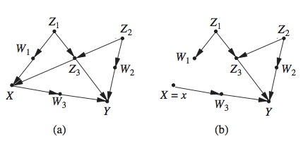
The second method mutilates the graph and uses the outcome node, Y, as a temporary surrogate for Y(x), with the understanding that the substitution is valid only under the mutilation. The mutilation required for this substitution is dictated by the First Law, and calls for removing all arrows entering the treatment variable X, as illustrated in the following graph (taken from here).

This method has some disadvantages compared with the first; the removal of X’s parents prevents us from seeing connections that might exist between Y_x and the pre-intervention treatment node X (as well as its descendants). To remedy this weakness, Shpitser and Pearl (2009) (link here) retained a copy of the pre-intervention X node, and kept it distinct from the manipulated X node.

Equivalently, Richardson and Robins (2013) spliced the X node into two parts, one to represent the pre-intervention variable X and the other to represent the constant X=x.

All in all, regardless of which variant you choose, the counterfactuals of interest can be represented as nodes in the structural graph, and inter-connections among these nodes can be used either to verify identification conditions or to facilitate algebraic operations in counterfactual logic.

Note, however, that all these variants stem from the First Law, Y(x) = Y[M_x], which DEFINES counterfactuals in terms of an operation on a structural equation model M.

Finally, to celebrate this “Flower of the First Law” and, thereby, the unification of the structural and potential outcome frameworks, I am posting a flowery photo of Don Rubin and myself, taken during Don’s recent visit to UCLA.

In several papers and lectures I have used the rhetorical title “The First Law of Causal Inference” when referring to the structural definition of counterfactuals:

The more I talk with colleagues and students, the more I am convinced that the equation deserves the title. In this post, I will explain why.

As many readers of Causality (Ch. 7) would recognize, Eq. (1) defines the potential-outcome, or counterfactual, Y_x(u) in terms of a structural equation model M and a submodel, M_x, in which the equations determining X is replaced by a constant X=x. Computationally, the definition is straightforward. It says that, if you want to compute the counterfactual Y_x(u), namely, to predict the value that Y would take, had X been x (in unit U=u), all you need to do is, first, mutilate the model, replace the equation for X with X=x and, second, solve for Y. What you get IS the counterfactual Y_x(u). Nothing could be simpler.

So, why is it so “fundamental”? Because from this definition we can also get probabilities on counterfactuals (once we assign probabilities, P(U=u), to the units), joint probabilities of counterfactuals and observables, conditional independencies over counterfactuals, graphical visualization of potential outcomes, and many more. [Including, of course, Rubin’s “science”, Pr(X,Y(0),(Y1))]. In short, we get everything that an astute causal analyst would ever wish to define or estimate, given that he/she is into solving serious problems in causal analysis, say policy analysis, or attribution, or mediation. Eq. (1) is “fundamental” because everything that can be said about counterfactuals can also be derived from this definition.
[See the following papers for illustration and operationalization of this definition:
http://ftp.cs.ucla.edu/pub/stat_ser/r431.pdf
http://ftp.cs.ucla.edu/pub/stat_ser/r391.pdf
http://ftp.cs.ucla.edu/pub/stat_ser/r370.pdf
also, Causality chapter 7.]

However, it recently occurred on me that the conceptual significance of this definition is not fully understood among causal analysts, not only among “potential outcome” enthusiasts, but also among structural equations researchers who practice causal analysis in the tradition of Sewall Wright, O.D. Duncan, and Trygve Haavelmo. Commenting on the flood of methods and results that emerge from this simple definition, some writers view it as a mathematical gimmick that, while worthy of attention, need to be guarded with suspicion. Others labeled it “an approach” that need be considered together with “other approaches” to causal reasoning, but not as a definition that justifies and unifies those other approaches.

Even authors who advocate a symbiotic approach to causal inference — graphical and counterfactuals — occasionally fail to realize that the definition above provides the logic for any such symbiosis, and that it constitutes in fact the semantical basis for the potential-outcome framework.

I will start by addressing the non-statisticians among us; i.e., economists, social scientists, psychometricians, epidemiologists, geneticists, metereologists, environmental scientists and more, namely, empirical scientists who have been trained to build models of reality to assist in analyzing data that reality generates. To these readers I want to assure that, in talking about model M, I am not talking about a newly invented mathematical object, but about your favorite and familiar model that has served as your faithful oracle and guiding light since college days, the one that has kept you cozy and comfortable whenever data misbehaved. Yes, I am talking about the equation

that you put down when your professor asked: How would household spending vary with income, or, how would earning increase with education, or how would cholesterol level change with diet, or how would the length of the spring vary with the weight that loads it. In short, I am talking about innocent equations that describe what we assume about the world. They now call them “structural equations” or SEM in order not to confuse them with regression equations, but that does not make them more of a mystery than apple pie or pickled herring. Admittedly, they are a bit mysterious to statisticians, because statistics textbooks rarely acknowledge their existence [Historians of statistics, take notes!] but, otherwise, they are the most common way of expressing our perception of how nature operates: A society of equations, each describing what nature listens to before determining the value it assigns to each variable in the domain.

Why am I elaborating on this perception of nature? To allay any fears that what is put into M is some magical super-smart algorithm that computes counterfactuals to impress the novice, or to spitefully prove that potential outcomes need no SUTVA, nor manipulation, nor missing data imputation; M is none other but your favorite model of nature and, yet, please bear with me, this tiny model is capable of generating, on demand, all conceivable counterfactuals: Y(0),Y(1), Y_x, Y_{127}, X_z, Z(X(y)) etc. on and on. Moreover, every time you compute these potential outcomes using Eq. (1) they will obey the consistency rule, and their probabilities will obey the laws of probability calculus and the graphoid axioms. And, if your model justifies “ignorability” or “conditional ignorability,” these too will be respected in the generated counterfactuals. In other words, ignorability conditions need not be postulated as auxiliary constraints to justify the use of available statistical methods; no, they are derivable from your own understanding of how nature operates.

In short, it is a miracle.

Not really! It should be self evident. Couterfactuals must be built on the familiar if we wish to explain why people communicate with counterfactuals starting at age 4 (“Why is it broken?” “Lets pretend we can fly”). The same applies to science; scientists have communicated with counterfactuals for hundreds of years, even though the notation and mathematical machinery needed for handling counterfactuals were made available to them only in the 20th century. This means that the conceptual basis for a logic of counterfactuals resides already within the scientific view of the world, and need not be crafted from scratch; it need not divorce itself from the scientific view of the world. It surely should not divorce itself from scientific knowledge, which is the source of all valid assumptions, or from the format in which scientific knowledge is stored, namely, SEM.

Here I am referring to people who claim that potential outcomes are not explicitly represented in SEM, and explicitness is important. First, this is not entirely true. I can see (Y(0), Y(1)) in the SEM graph as explicitly as I see whether ignorability holds there or not. [See, for example, Fig. 11.7, page 343 in Causality]. Second, once we accept SEM as the origin of potential outcomes, as defined by Eq. (1), counterfactual expressions can enter our mathematics proudly and explicitly, with all the inferential machinery that the First Law dictates. Third, consider by analogy the teaching of calculus. It is feasible to teach calculus as a stand-alone symbolic discipline without ever mentioning the fact that y'(x) is the slope of the function y=f(x) at point x. It is feasible, but not desirable, because it is helpful to remember that f(x) comes first, and all other symbols of calculus, e.g., f'(x), f”(x), [f(x)/x]’, etc. are derivable from one object, f(x). Likewise, all the rules of differentiation are derived from interpreting y'(x) as the slope of y=f(x).

Where am I heading?
First, I would have liked to convince potential outcome enthusiasts that they are doing harm to their students by banning structural equations from their discourse, thus denying them awareness of the scientific basis of potential outcomes. But this attempted persuasion has been going on for the past two decades and, judging by the recent exchange with Guido Imbens (link), we are not closer to an understanding than we were in 1995. Even an explicit demonstration of how a toy problem would be solved in the two languages (link) did not yield any result.

Second, I would like to call the attention of SEM practitioners, including of course econometricians, quantitative psychologists and political scientists, and explain the significance of Eq. (1) in their fields. To them, I wish to say: If you are familiar with SEM, then you have all the mathematical machinery necessary to join the ranks of modern causal analysis; your SEM equations (hopefully in nonparametric form) are the engine for generating and understanding counterfactuals.; True, your teachers did not alert you to this capability; it is not their fault, they did not know of it either. But you can now take advantage of what the First Law of causal inference tells you. You are sitting on a gold mine, use it.

Finally, I would like to reach out to authors of traditional textbooks who wish to introduce a chapter or two on modern methods of causal analysis. I have seen several books that devote 10 chapters on SEM framework: identification, structural parameters, confounding, instrumental variables, selection models, exogeneity, model misspecification, etc., and then add a chapter to introduce potential outcomes and cause-effect analyses as useful new comers, yet alien to the rest of the book. This leaves students to wonder whether the first 10 chapters were worth the labor. Eq. (1) tells us that modern tools of causal analysis are not new comers, but follow organically from the SEM framework. Consequently, one can leverage the study of SEM to make causal analysis more palatable and meaningful.

Please note that I have not mentioned graphs in this discussion; the reason is simple, graphical modeling constitutes The Second Law of Causal Inference.

Enjoy both,
Judea

In a recent posting on this blog, Elias and Bryant described how graphical methods can help decide if a pseudo-randomized variable, Z, qualifies as an instrumental variable, namely, if it satisfies the exogeneity and exclusion requirements associated with the definition of an instrument. In this note, I aim to describe how inferences of this type can be performed without graphs, using the language of potential outcome. This description should give students of causality an objective comparison of graph-less vs. graph-based inferences. See my exchange with Guido Imbens [here].

Every problem of causal inference must commence with a set of untestable, theoretical assumptions that the modeler is prepared to defend on scientific grounds. In structural modeling, these assumptions are encoded in a causal graph through missing arrows and missing latent variables. Graphless methods encode these same assumptions symbolically, using two types of statements:

1. Exclusion restrictions, and
2. Conditional independencies among observable and potential outcomes.

For example, consider the causal Markov chain which represents the structural equations:

with and being omitted factors such that X, , are mutually independent.

These same assumptions can also be encoded in the language of counterfactuals, as follows:

(3) represents the missing arrow from X to Z, and (4)-(6) convey the mutual independence of X, , and .
[Remark: General rules for translating graphical models to counterfactual notation are given in Pearl (2009, pp. 232-234).]

Assume now that we are given the four counterfactual statements (3)-(6) as a specification of a model; What machinery can we use to answer questions that typically come up in causal inference tasks? One such question is, for example, is the model testable? In other words, is there an empirical test conducted on the observed variables X, Y, and Z that could prove (3)-(6) wrong? We note that none of the four defining conditions (3)-(6) is testable in isolation, because each invokes an unmeasured counterfactual entity. On the other hand, the fact the equivalent graphical model advertises the conditional independence of X and Z given Y, X _||_ Z | Y, implies that the combination of all four counterfactual statements should yield this testable implication.

Another question often posed to causal inference is that of identifiability, for example, whether the
causal effect of X on Z is estimable from observational studies.

Whereas graphical models enjoy inferential tools such as d-separation and do-calculus, potential-outcome specifications can use the axioms of counterfactual logic (Galles and Pearl 1998, Halpern, 1998) to determine identification and testable implication. In a recent paper, I have combined the graphoid and counterfactual axioms to provide such symbolic machinery (link).

However, the aim of this note is not to teach potential outcome researchers how to derive the logical consequences of their assumptions but, rather, to give researchers the flavor of what these derivation entail, and the kind of problems the potential outcome specification presents vis a vis the graphical representation.

As most of us would agree, the chain appears more friendly than the 4 equations in (3)-(6), and the reasons are both representational and inferential. On the representational side we note that it would take a person (even an expert in potential outcome) a pause or two to affirm that (3)-(6) indeed represent the chain process he/she has in mind. More specifically, it would take a pause or two to check if some condition is missing from the list, or whether one of the conditions listed is redundant (i.e., follows logically from the other three) or whether the set is consistent (i.e., no statement has its negation follows from the other three). These mental checks are immediate in the graphical representation; the first, because each link in the graph corresponds to a physical process in nature, and the last two because the graph is inherently consistent and non-redundant. As to the inferential part, using the graphoid+counterfactual axioms as inference rule is computationally intractable. These axioms are good for confirming a derivation if one is proposed, but not for finding a derivation when one is needed.

I believe that even a cursory attempt to answer research questions using (3)-(5) would convince the reader of the merits of the graphical representation. However, the reader of this blog is already biased, having been told that (3)-(5) is the potential-outcome equivalent of the chain X—>Y—>Z. A deeper appreciation can be reached by examining a new problem, specified in potential- outcome vocabulary, but without its graphical mirror.

Assume you are given the following statements as a specification.

It represents a familiar model in causal analysis that has been throughly analyzed. To appreciate the power of graphs, the reader is invited to examine this representation above and to answer a few questions:

a) Is the process described familiar to you?
b) Which assumption are you willing to defend in your interpretation of the story.
c) Is the causal effect of X on Y identifiable?
d) Is the model testable?

I would be eager to hear from readers
1. if my comparison is fair.
2. which argument they find most convincing.

A recent article by Heckman and Pinto (HP) (link: http://www.nber.org/papers/w19453.pdf) discusses the do-calculus as a formal operationalization of Haavelmo’s approach to policy intervention. HP replace the do-operator with an equivalent operator, called “fix,” which simulates a Fisherian experiment with randomized “do”. They advocate the use of “fix,” discover limitations in “do,” and inform readers that those limitations disappear in “the Haavelmo approach.”

I examine the logic of HP’s paper, its factual basis, and its impact on econometric research and education (link: http://ftp.cs.ucla.edu/pub/stat_ser/r420.pdf).

David Kenny’s website <http://davidakenny.net/cm/mediate.htm> has recently been revised to include a section on the Causal Inference Approach to Mediation. As many readers know, Kenny has pioneered mediation analysis in the social sciences through his seminal papers with Judd (1981) and Baron(1986) and has been an active leader in this field. His original approach, often referred to as the “Baron and Kenny (BK) approach,” is grounded in conservative Structural Equation Modeling (SEM) analysis, in which causal relationships are asserted with extreme caution and the boundaries between statistical and causal notions vary appreciably among researchers.

It is very significant therefore that Kenny has decided to introduce causal mediation analysis to the community of SEM researchers which, until very recently, felt alienated from recent advances in causal mediation analysis, primarily due to the counterfactual vocabulary in which it was developed and introduced. With Kenny’s kind permission, I am posting his description below, because it is one of the few attempts to explain causal inference in the language of traditional SEM mediation analysis and, thus, it may serve to bridge the barriers between the two communities.

Next you can find Kenny’s new posting, annotated with my comments. In these comments, I have attempted to further clarify the bridges between the two cultures; the “traditional” and the “causal.” I will refer to the former as “BK” (for Baron and Kenny) and to the latter as “causal” (for lack of a better word) although, conceptually, both BK and SEM are fundamentally causal.

Click here for the full post.

Larry Wasserman posted the following comments on his “normal-deviate” blog:
http://normaldeviate.wordpress.com/2013/08/09/the-jsm-minimaxity-and-the-language-police/

I am back from the JSM (http://www.amstat.org/meetings/jsm/2013/). For those who don’t know, the JSM is the largest statistical meeting in the world. This year there were nearly 6,000 people.

*******skipping *******
On Tuesday, I went to Judea Pearl’s medallion lecture, with discussions by Jamie Robins and Eric Tchetgen Tchetgen. Judea gave an unusual talk, mixing philosophy, metaphors (eagles and snakes can’t build microscopes) and math. Judea likes to argue that graphical models/structural equation models are the best way to view causation. Jamie and Eric argued that graphs can hide certain assumptions and that counterfactuals need to be used in addition to graphs.
***********more *********

J. Pearl:

I posted the following reply:

Larry,

Your note about my Medallion Lecture (at JSM 2013) may create the impression that I am against the use of counterfactuals.

This is not the case.

1. I repeatedly say that counterfactuals are the building blocks of rational behavior and scientific thoughts.
see: http://ftp.cs.ucla.edu/pub/stat_ser/R269.pdf
http://ftp.cs.ucla.edu/pub/stat_ser/r360.pdf

2. I showed that ALL counterfactuals can be encoded parsimoniously in one structural equation model, and can be read easily from any such model.
see: http://ftp.cs.ucla.edu/pub/stat_ser/r370.pdf

3. I showed how the graphical-counterfactual symbiosis can work to unleash the merits of both. And I emphasized that mediation analysis would still be in its infancy if it were not for the algebra of counterfactuals (as it emerges from structural semantics.)

4. I am aware of voiced concerns about graphs hiding assumptions, but I prefer to express these concerns in terms of “hiding opportunities”, rather than “hiding assumptions” because the latter is unnecessarily alarming.

A good analogy would be Dawid’s notation X||Y for independence among variables, which states that every event of the form X = x_i is independent of every event of the form Y=y_j. There may therefore be hundreds of assumptions conveyed by the innocent and common statement X||Y.

Is this a case of hiding assumptions?
I do not believe so.

Now imagine that we are not willing to defend the assumption “X = x_k is independent of Y=y_m” for some specific k and m. The notation forces us to write “variable X is not independent of variable Y” thus hiding all the (i,j) pairs for which the independence is defensible. This is a loss of opportunity, not a hiding of assumptions, because refraining from assuming independence is a more conservative strategy; it prevents unwarranted conclusions from being drawn.

Thanks for commenting on my lecture.

We received the following query from Jim Grace, (USGS – National Wetlands Research Center) :
Hi Judea,

In your 2009 edition of Causality on pages 26-27 you explain your reasoning for now preferring to express causal rules from a Laplacian quasi-deterministic perspective rather than stay with the stochastic conceptualization associated with Bayesian Networks. It seems to me that a practical matter here is the reliance of traditional graph theory on discrete mathematics and the constraints that places on functional forms and, therefore, counterfactual arguments. Despite that clear logic, one sees the occasional discussion of “causal Bayes nets” and I wondered if you would dissuade people (if people can be dissuaded) from trying to evolve a causal modeling methodology with discrete Bayes nets as their starting point?

Judea Pearl answers:
Dear Jim,

I would not dissuade people from using either causal Bayesian causal networks or structural equation models, because the difference between the two is so minute that it is not worth the dissuasion. The question is only what question you ask yourself when you construct the diagram. If you feel more comfortable asking: What factors determine the value of this variable” then you construct a structural equation model. If on the other hand you prefer to ask: “If I intervene and wiggle this variable, would the probability of the other variable change?” then the outcome would be a causal Bayes network. Rarely do they differ (but see example on page 35 of Causality).

We received the following query from Megan Murphy (ASA):
Dr. Pearl,
I received the following question regarding the Causality in Statistics Education prize on twitter. I’m not sure how to answer this, perhaps you can help?

Would entries using Neyman-Rubin model even be considered? RT @AmstatNews: Causality in Statistics Education #prize magazine.amstat.org/blog/2012/11/0…

Judea Answers:
“Of course! The criteria for evaluation specifically state: ‘in some mathematical language (e.g., counterfactuals, equations, or graphs)’ giving no preference to any of the three notational systems. The criteria stress capabilities to perform specific inference tasks, regardless of the tools used in performing the tasks.

For completeness, I re-list below the evaluation criteria:

• The extent to which the material submitted equips students with skills needed for effective causal reasoning. These include:

—1a. Ability to correctly classify problems, assumptions, and claims into two distinct categories: causal vs. associational

—1b. Ability to take a given causal problem and articulate in some mathematical language (e.g., counterfactuals, equations, or graphs) both the target quantity to be estimated and the assumptions one is prepared to make (and defend) to facilitate a solution

—1c. Ability to determine, in simple cases, whether control for covariates is needed for estimating the target quantity, what covariates need be controlled, what the resulting estimand is, and how it can be estimated using the observed data

—1d. Ability to take a simple scenario (or model), determine whether it has statistically testable implications, and apply data to test the assumed scenario

• The extent to which the submitted material assists statistics instructors in gaining an understanding of the basics of causal inference (as outlined in 1a-d) and prepares them to teach these basics in undergraduate and lower-division graduate classes in statistics.

Those versed in the Neyman-Rubin model are most welcome to submit nominations.

Note, however, that nominations will be evaluated on ALL four skills, 1a – 1d.
Judea

I recently attended a seminar presentation by Professor Tom Belin, (AQM RAC seminar, UCLA, November 30, 2012) who spoke on the relationships between the potential outcome model of Neyman, Rubin and Holland, and the structural equation and graphical models which I have been advocating since 1995.

In the last part of the seminar, I made a few comments which led to a lively discussion, as well as clarification ( I hope) of some basic issues which are rarely discussed in the mainstream literature.

Below is a concise summary of my remarks which I present to encourage additional discussion, questions, objections and, of course, new ideas.

Judea Pearl

Summary of my views on the relationships between the potential-outcome (PO) and Structural Causal Models (SCM) frameworks.

Formally, the two frameworks are logically equivalent; a theorem in one is a theorem in the other, and every assumption in one can be translated into an equivalent assumption in the other.

Therefore, the two frameworks can be used interchangeably and symbiotically, as it is done in the advanced literature in the health and social sciences.

However, the PO framework has also spawned an ideological movement that resists this symbiosis and discourages its faithfuls from using SCM or its graphical representation.

This ideological movement (which I call “arrow-phobic”) can be recognized by a total avoidance of causal diagrams or structural equations in research papers, and an exclusive use of “ignorability” type notation for expressing the assumptions that (must) underlie causal inference studies. For example, causal diagrams are meticulously excluded from the writings of Rubin, Holland, Rosenbaum, Angrist, Imbens, and their students who, by and large, are totally unaware of the inferential and representational powers of diagrams.

Formally, this exclusion is harmless because, based on the logical equivalence mentioned above, it is always possible to replace assumptions made in SCM with equivalent, albeit cumbersome assumptions in PO language, and eventually come to the correct conclusions. But practically, the exclusion forces investigators to articulate assumptions whose meaning they do not comprehend, whose plausibility they cannot judge, and whose statistical implications they cannot predict.

The arrow-phobic exclusion can be compared to a prohibition against the use of ‘multiplication’ in arithmetics. Formally, it is harmless, because one can always replace multiplication with addition (e.g., adding a number to itself n times). Yet practically, those who shun multiplication will not get very far in science.

The rejection of graphs and structural models leaves investigators with no process-model guidance and, not surprisingly, it has resulted in a number of blunders which the PO community is not very proud of.

One such blunder is Rosenbaum (2002) and Rubin’s (2007) declaration that “there is no reason to avoid adjustment for a variable describing subjects before treatment”
http://www.cs.ucla.edu/~kaoru/r348.pdf

Another is Hirano and Imbens’ (2001) method of covariate selection, which prefers bias-amplifying variables in the propensity score.
http://ftp.cs.ucla.edu/pub/stat_ser/r356.pdf

The third is the use of ‘principal stratification’ to assess direct and indirect effects in mediation problems. which lead to paradoxical and unintended results.
http://ftp.cs.ucla.edu/pub/stat_ser/r382.pdf

In summary, the PO framework offers a useful analytical tool (i.e.. an algebra of counterfactuals) when used in the context of a symbiotic SCM analysis. It may be harmful however when used as an exclusive and restrictive subculture that discourages the use of process-based tools and insights.

Additional background and technical details on the PO vs. SCM tradeoffs can be found in Section 4 of a tutorial paper (Statistics Surveys)
http://ftp.cs.ucla.edu/pub/stat_ser/r350.pdf
and in a book chapter on the Eight Myths of SEM:
http://ftp.cs.ucla.edu/pub/stat_ser/r393.pdf

Readers might also find it instructive to compare how the two paradigms frame and solve a specific problem from start to end. This comparison is given in Causality (Pearl 2009) pages 81-88, 232-234.