Causal Analysis in Theory and Practice » 2023

March 17, 2023

Personalized Decision Making under Concurrent-Controlled RCT Data

Filed under: Uncategorized — Scott Mueller @ 2:31 am

Scott Mueller and Judea Pearl

Introduction

This note supplements the analysis of [Mueller and Pearl 2023] by introducing an important restriction on the data obtained from Randomized Control Trials (RCT). In Mueller and Pearl, it is assumed that RCTs provide estimates of two probabilities, $P(y_t)$ and $P(y_c)$, standing for the probability of the outcome $Y$ under treatment and control, respectively. In medical practices, however, these two quantities are rarely reported separately; only their difference $\text{ATE} = P(y_t)-P(y_c)$ is measured, estimated, and reported. The reason is that the individual effects, $P(y_t)$ and $P(y_c)$, are suspect of contamination by selection bias and placebo effects. These two imperfections are presumed to cancel out by a method called “Concurrent Control” [Senn 2010] in which subjects in both treatment and control arms are measured simultaneously and only the average difference, ATE, is counted¹.

This note establishes bounds on $P(\text{benefit})$ and $P(\text{harm})$ under the restriction that RCTs provide only an assessment of ATE, not of the individual causal effects $P(y_t)$ and $P(y_c)$. We will show that the new restriction, though leading to wider bounds, still permits the extraction of meaningful information on individual harm and benefit and, when combined with observational data, can be extremely valuable in personalized decision making.

Our results can be summarized in the following two inequalities. The first inequality bounds PNS (same as $P(\text{benefit})$) without observational data, and the second bounds PNS using both ATE and observational data in the form of $P(X, Y)$.

With just the ATE, PNS is bounded as:

$$\begin{equation} \max\{0, \text{ATE}\} \leqslant \text{PNS} \leqslant \min\{1, \text{ATE} + 1\}. \end{equation}$$

The lower bound is above zero when ATE is positive, and the upper bound is lower than 1 when ATE is negative.

When we combine ATE with observational data, the lower bound remains the same, but the upper bound changes to yield:

$$\begin{equation} \max\{0, \text{ATE}\} \leqslant \text{PNS} \leqslant \min\left\{\begin{array}{r} P(x,y) + P(x’,y’),\\ \text{ATE} + P(x, y’) + P(x’, y) \end{array}\right\}. \end{equation}$$

The upper bound in (2), is always lower than (or equal to) the one in (1), because both $P(x,y) + P(x’,y’) \leqslant 1$ and $P(x, y’) + P(x’, y) \leqslant 1$.

In Appendix we will present the derivations of Eqs. (1) and (2), whereas in the following section, we discuss some of their ramifications.

Footnote

1: See footnote 11 in [Mueller and Pearl 2023] and [Pearl 2013] for ways in which selection bias can be eliminated when linearity is assumed (after scaling).

How observational data inform PNS (or P(benefit))

The bounds on PNS produced by Eqs. (1) and (2) can be visualized interactively². To show the contrast between Eq. (1) and Eq. (2), Fig. 1 displays the allowable values of PNS for various levels of ATE, assuming no observational information is available (i.e., Eq. (1)). We see, for example, that for $\text{ATE} = 0$ (left vertical dashed line), the bound is vacuous ($0 \leqslant \text{PNS} \leqslant 1$), while for $\text{ATE}=0.5$ (right vertical dashed line), we have $\frac12 \leqslant \text{PNS} \leqslant 1$ — a somewhat more informative bound, but still rather trivial.

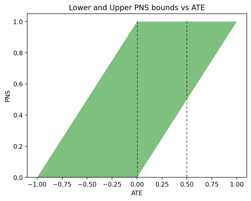
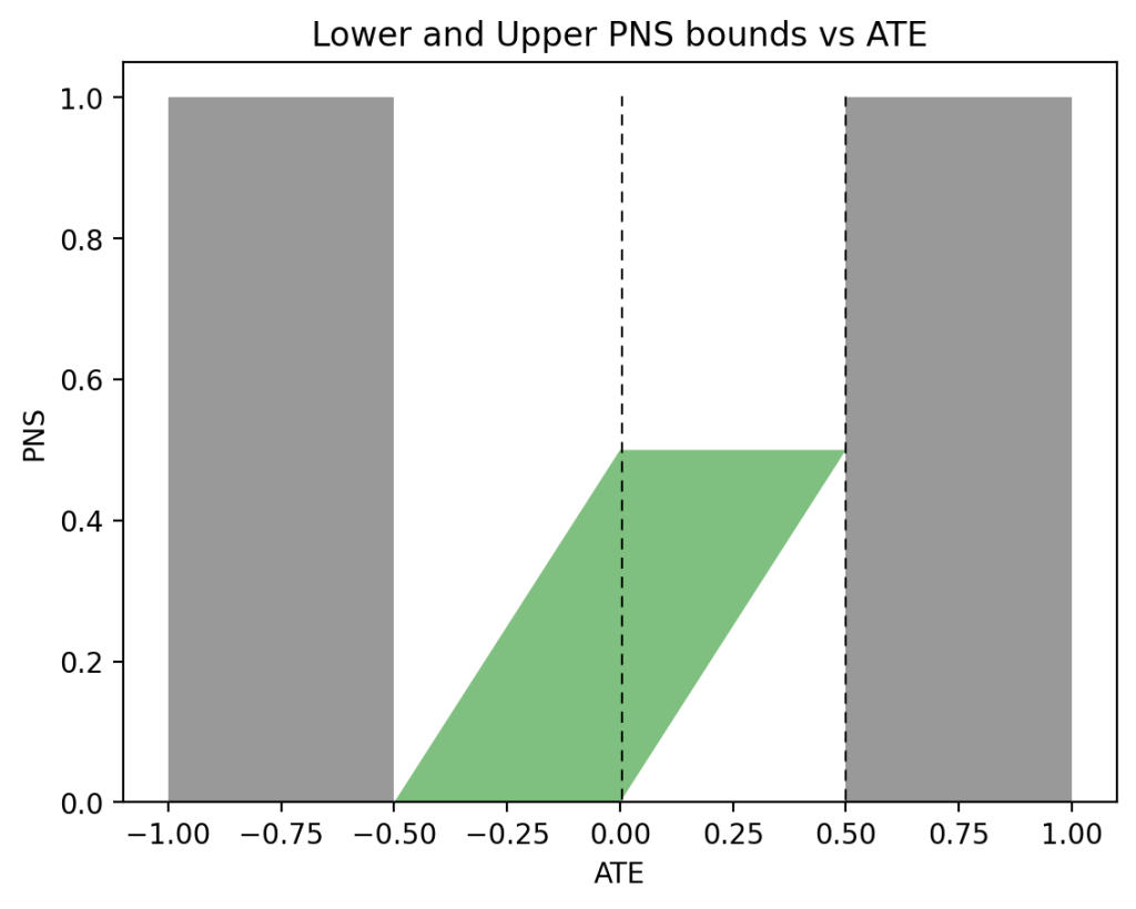
Figure 1: The green area represents possible PNS values for the given ATE, while the white areas represent values not achievable by PNS.

Figure 2 displays the allowable values of PNS when observational data are available. We see that for $\text{ATE} = 0$ (left vertical dashed line), we now have $0 \leqslant \text{PNS} \leqslant \frac12$, whereas for $\text{ATE} = 0.5$ (right vertical dashed line), we now have a point estimate $\text{PNS} = \frac12$, assuring us that exactly 50\% of all subjects will benefit from the treatment (and none will be harmed by it).

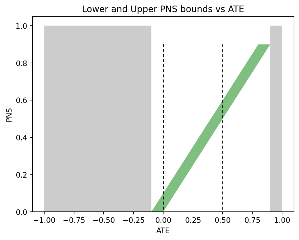
Figure 2: The green area represents possible PNS values for the given ATE, while the gray areas represent values of ATE that are incompatible with the assumed observational information: P(y|x) = P(y|x’) = P(x) = 0.5.

When observational data become less symmetric, say $P(x)=0.5$, $P(y|x)=0.9$, and $P(y|x’)=0.1$, the regions of possible and impossible PNS values shift significantly. Moving the sliders for $P(x)$, $P(y|x)$, and $P(y|x’)$ to the above values produces the graph shown in Figure 3. This time, when $\text{ATE} = 0$ (left vertical dashed line), the bounds on PNS narrow down to $0 \leqslant \text{PNS} \leqslant 0.1$, telling us that subjects have a maximum 10\% chance of benefiting from the treatment. When $\text{ATE}=0.5$ (right vertical dashed line), we have $\frac12 \leqslant \text{PNS} \leqslant 0.6$, still a narrow width of $0.1$, with an assurance of at least 50\% chance of benefiting from the treatment.

It should be clear now that consequential information on individual benefit can be obtained even when separate causal effects, $P(y_x)$ and $P(y_{x’})$, are unavailable. The same situation holds for $P(\text{harm})$ as well.

Figure 3: The green area represents possible PNS values for the given ATE and observational probabilities: P(x) = 0.5, P(y|x) = 0.9, P(y|x’) = 0.1.

Footnote

2: Visualization is at https://ate-bounds.streamlit.app.

How Observational Data inform the Probability of Harm P(harm)

The probability of harm is the converse of PNS. We can bound this probability with ATE and with observational data similar to Eqs. (1) and (2). With just the ATE, $P(\text{harm})$ is bounded as:

$$\begin{equation} \max\{0, -\text{ATE}\} \leqslant \text{PNS} \leqslant \min\{1, 1 – \text{ATE}\}. \end{equation}$$

The lower bound is positive when ATE is positive, and the upper bound is less than $1$ when ATE is negative. When we combine observational data, a smaller upper bound is possible:

$$\begin{equation} \max\{0, \text{ATE}\} \leqslant \text{PNS} \leqslant \min\left\{\begin{array}{r} P(x,y’) + P(x’,y),\\ P(x, y) + P(x’, y’) – \text{ATE} \end{array}\right\}. \end{equation}$$

Again, the upper bound in (4), is always lower than (or equal to) the one in (3), since $P(x,y) + P(x’,y’) \leqslant 1$ and $P(x, y’) + P(x’, y) \leqslant 1$. See Appendix for the derivations of Eqs. (3) and (4).

Figures 4a and 4b depict these bounds under the same conditions as Figures 1 and 2, respectively.

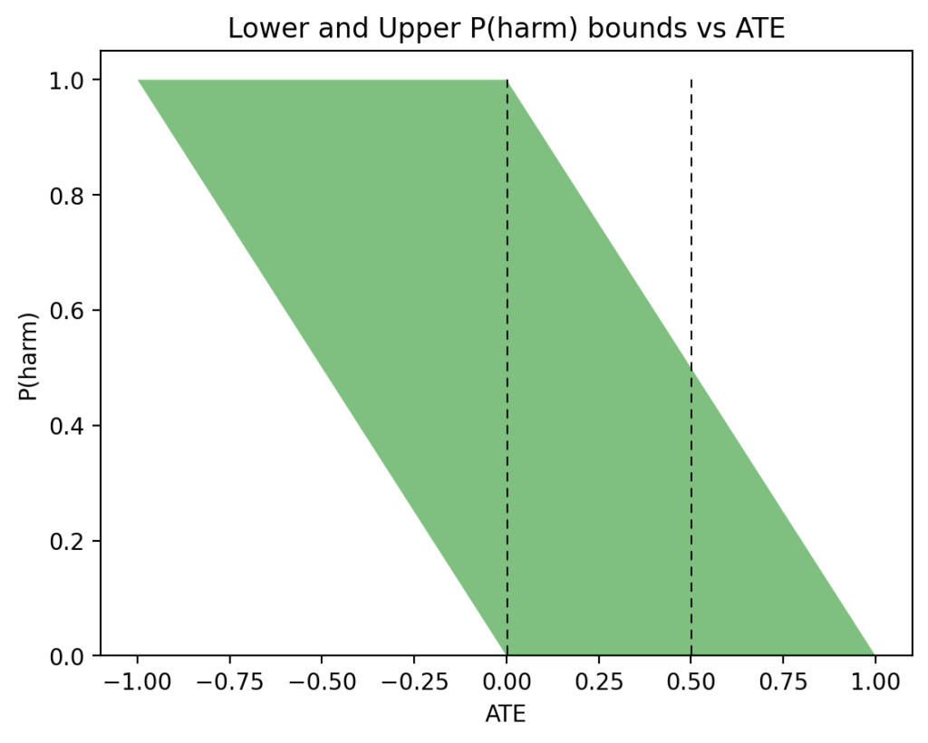
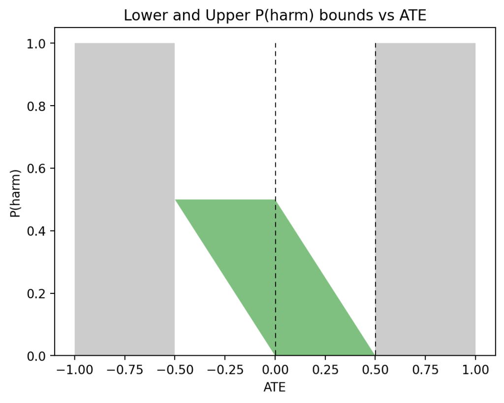
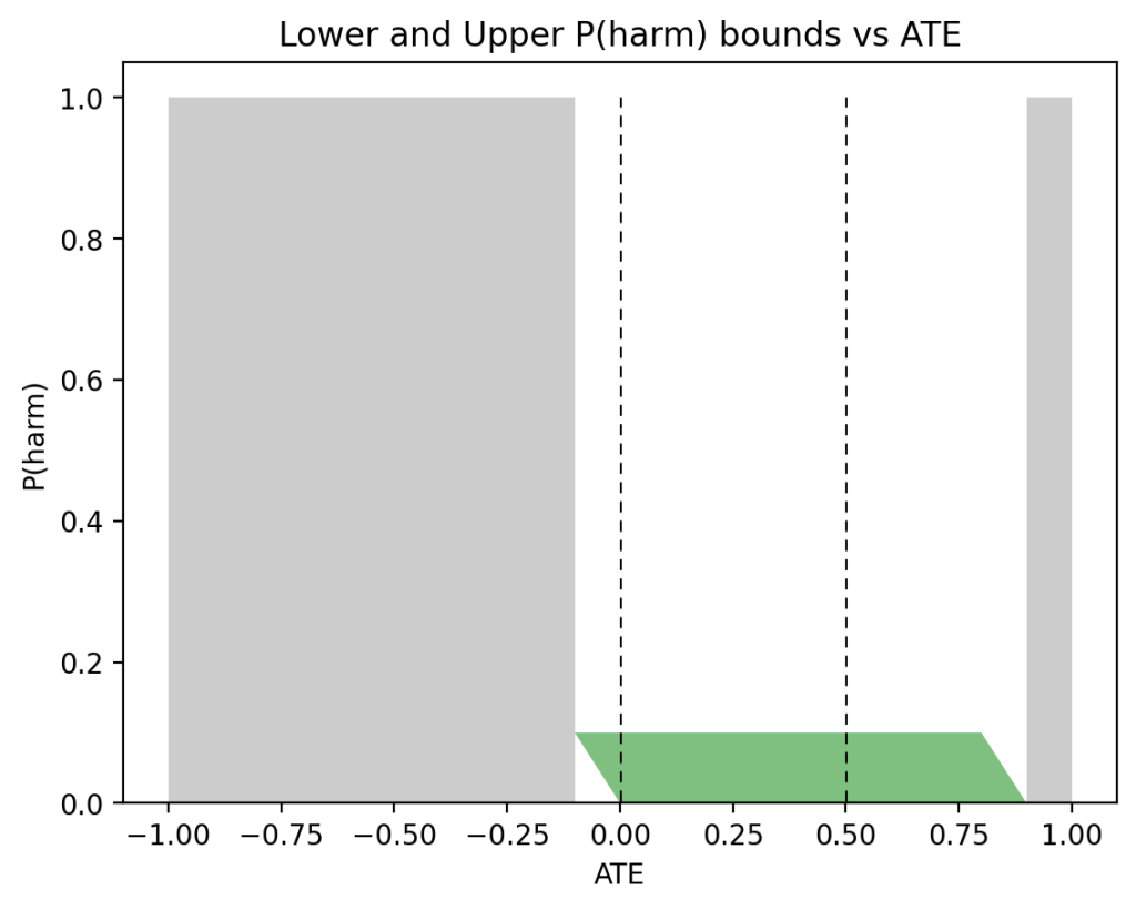
Figure 4: P(harm) graphs corresponding to Figures 1 and 2 for PNS.

Figure 5, on the other hand, shows very different sets of bounds for the asymmetric case: $P(x) = 0.5$, $P(y|x) = 0.9$, and $P(y|x’) = 0.1$, used in Figure 3. This time, $0 \leqslant P(\text{harm}) \leqslant 0.1$ when $\text{ATE}=0$ or $\text{ATE}=0.5$. This has the same width of $0.1$ as in the case of PNS, but with a substantially different shape.

Figure 5: The green area represents possible P(harm) values for the given ATE and observational probabilities: P(x)= 0.5, P(y|x) = 0.9, P(y|x’) = 0.1.

Intuition

The intuition behind the PNS lower bound is that the probability of benefiting cannot be less than the positive part of the difference in causal effects. That difference must be explained by benefiting from treatment.

The intuition behind the PNS upper bound is split into two parts. First, the benefiters must be among the individuals who chose treatment and had a successful outcome, $(x, y)$, or those who avoided treatment and had an unsuccessful outcome, $(x’, y’)$. Therefore, one potential upper bound is $P(x,y) + P(x’,y’)$. Alternatively, since $\text{ATE} = \text{PNS} – P(\text{harm})$, we get an upper bound on PNS by adding at least the proportion of individuals harmed to ATE. This is precisely the upper bound $\text{ATE} + P(x, y’) + P(x’, y)$ because the proportion of individuals choosing treatment and having an unsuccessful outcome, $P(x, y’)$, and the proportion of individuals avoiding treatment and having a successful outcome, $P(x’, y)$, comprise all individuals harmed by treatment as well as some additional individuals.

Similar reasoning holds for the lower and upper bounds of $P(\text{harm})$.

Bounds on ATE

In addition to informing PNS and $P(\text{harm})$, observational data also impose restrictions on ATE, violations of which imply experimental imperfections. We start with Tian and Pearl’s bounds on causal effects [Tian and Pearl 2000]:

$$\begin{align} P(x,y) &\leqslant P(y_x) \leqslant 1 – P(x, y’),\\ P(x’,y) &\leqslant P(y_{x’}) \leqslant 1 – P(x’, y’). \end{align}$$

If we multiply Equation (6) by $-1$ and add it to Equation (5), we get the following bounds on ATE:

$$\begin{align} P(x,y) + P(x’,y’) – 1 &\leqslant \text{ATE} \leqslant P(x,y) + P(x’,y’). \end{align}$$

While the range of ATE values has a width of $1$, the location of this range can still alert the experimenter to possible incompatibilities between the observational and experimental data.

Appendix

The lower and upper bounds in Equation (2) follow directly from the Tian-Pearl bounds on PNS. There are two additional possible lower bounds on PNS: $P(y_x) – P(y)$ and $P(y) – P(y_{x’})$. Since $P(y_x) – P(y) = \text{ATE} + P(y_{x’}) – P(y)$ and $P(y_{x’}) \geqslant 0$, a potential lower bound of $\text{ATE} – P(y)$ could be added to the $\max$ function of the left inequality (2). However, the existing lower bound $\text{ATE}$ subsumes it because $P(y) \geqslant 0$. Similarly, since $P(y) – P(y_{x’}) = \text{ATE} – P(y_x) + P(y)$ and $P(y_x) \leqslant 1$, a potential lower bound of $\text{ATE} – P(y’)$ could be added to inequalities (2). Again, the existing lower bound $\text{ATE}$ subsumes it.

There are two additional possible upper bounds on PNS: $P(y_x)$ and $P(y’_{x’})$. Since $P(y_x) = \text{ATE} + P(y_{x’})$ and $P(y_{x’}) \leqslant 1$, a potential upper bound of $\text{ATE} + 1$ could be added to the $\min$ function of the right inequality (2). However, the existing upper bound $\text{ATE} + P(x, y’) + P(x’, y)$ subsumes it because $P(x, y’) + P(x’, y) \leqslant 1$. Similarly, since $P(y’_{x’}) = \text{ATE} + 1 – P(y_x) = \text{ATE} + P(y’_x)$ and $P(y’_x) \leqslant 1$, a potential upper bound of $\text{ATE} + 1$ could be added to inequalities (2). Again, the existing upper bound $\text{ATE} + P(x, y’) + P(x’, y)$ subsumes it.

It may appear that the upper bound might dip below the lower bound, which would be problematic. In particular, either of the following two cases would cause this situation:

$$\begin{align} P(x,y) + P(x’,y’) &< \text{ATE}, \text{or}\\ \text{ATE} + P(x,y') + P(x',y) &< 0. \end{align}$$

Neither of these inequalities can occur because of the inequalities in (7). Inequality (8) cannot occur because of the right inequality of (7). Similarly, inequality (9) cannot occur because of the left inequality of (7).

References

Mueller, Scott and Judea Pearl (2023). “Personalized Decision Making – A Conceptual Introduction”. In: Journal of Causal Inference. url: http://ftp.cs.ucla.edu/pub/stat_ser/r513.pdf.
Pearl, Judea (May 29, 2013). “Linear Models: A Useful “Microscope” for Causal Analysis”. In: Journal of Causal Inference 1.1, pp. 155–170. issn: 2193-3685, 2193-3677. doi: 10.1515/jci-2013-0003. url: https://www.degruyter.com/document/doi/10.1515/jci-2013-0003/html (visited on 03/16/2023).
Senn, Stephen (2010). “Control in Clinical Trials”. In: Proceedings of the Eighth International Conference on Teaching Statistics. url: https://iase-web.org/documents/papers/icots8/ICOTS8_6D2_SENN.pdf.
Tian, Jin and Judea Pearl (2000). “Probabilities of causation: Bounds and identification”. In: Annals of Mathematics and Artificial Intelligence 28.1-4, pp. 287–313. url: http://ftp.cs.ucla.edu/pub/stat_ser/r271-A.pdf.

Comments (0)