Causal Inference (CI) − A year in review
2022 has witnessed a major upsurge in the status of CI, primarily in its general recognition as an independent and essential component in every aspect of intelligent decision making. Visible evidence of this recognition were several prestigious prizes awarded explicitly to CI-related research accomplishments. These include (1) the Nobel Prize in economics, awarded to David Card, Joshua Angrist, and Guido Imbens for their works on cause and effect relations in natural experiments https://www.nobelprize.org/prizes/economic-sciences/2021/press-release/ (2) The BBVA Frontiers of Knowledge Award to Judea Pearl for “laying the foundations of modern AI” https://www.eurekalert.org/news-releases/942893 and (3) The Rousseeuw Prize for Statistics to Jamie Robins, Thomas Richardson, Andrea Rotnitzky, Miguel Hernán, and Eric Tchetchgen Tchetchgen, for their “pioneering work on Causal Inference with applications in Medicine and Public Health” https://www.rousseeuwprize.org/news/winners-2022.
w
My acceptance speech at the BBVA award can serve as a gentle summary of the essence of causal inference, its basic challenges and major achievements: https://www.youtube.com/watch?v=uaq389ckd5o.
It is not a secret that I have been critical of the approach Angrist and Imbens are taking in econometrics, for reasons elaborated here https://ucla.in/2FwdsGV, and mainly here https://ucla.in/36EoNzO. I nevertheless think that their selection to receive the Nobel Prize in economics is a positive step for CI, in that it calls public attention to the problems that CI is trying to solve and will eventually inspire curious economists to seek a more broad-minded approach to these problems, so as to leverage the full arsenal of tools that CI has developed.
Coupled with these highlights of recognition, 2022 has seen a substantial increase in CI activities on both the academic and commercial fronts. The number of citations to CI related articles has reached a record high of over 10,200 citations in 2022, https://scholar.google.com/citations?user=bAipNH8AAAAJ&hl=en , showing positive derivatives in all CI categories. Dozens, if not hundreds of seminars, workshops and symposia have been organized in major conferences to disseminate progress in CI research. New results on individualized decision making were prominently featured in these meetings (e.g., https://ucla.in/33HSkNI). Several commercial outfits have come up with platforms for CI in their areas of specialization, ranging from healthcare to finance and marketing. (Company names such as #causallense, and Vianai Systems come to mind:
https://www.causalens.com/startup-series-a-funding-round-45-million/, https://arxiv.org/ftp/arxiv/papers/2207/2207.01722.pdf). Naturally, these activities have led to increasing demands for trained researchers and educators, versed in the tools of CI; jobs openings explicitly requiring experience in CI have become commonplace in both industry and academia.
I am also happy to see CI becoming an issue of contention in AI and Machine Learning (ML), increasingly recognized as an essential capability for human-level AI and, simultaneously, raising the question of whether the data-fitting methodologies of Big Data and Deep Learning could ever acquire these capabilities. In https://ucla.in/3d2c2Fi I’ve answered this question in the negative, though various attempts to dismiss CI as a species of “inductive bias” (e.g., https://www.youtube.com/watch?v=02ABljCu5Zw) or “missing data problem” (e.g., https://www.jstor.org/stable/pdf/26770992.pdf) are occasionally being proposed as conceptualizations that could potentially replace the tools of CI. The Ladder of Causation tells us what extra-data information would be required to operationalize such metaphorical aspirations.
Researchers seeking a gentle introduction to CI are often attracted to multi-disciplinary forums or debates, where basic principles are compiled and where differences and commonalities among various approaches are compared and analyzed by leading researchers. Not many such forums were published in 2022, perhaps because the differences and commonalities are now well understood or, as I tend to believe, CI and its Structural Causal Model (SCM) unifies and embraces all other approaches. I will describe two such forums in which I participated.
(1) In March of 2022, the Association for Computing Machinery (ACM) has published an anthology containing highlights of my works (1980-2020) together with commentaries and critics from two dozens authors, representing several disciplines. The Table of Content can be seen here: https://ucla.in/3hLRWkV. It includes 17 of my most popular papers, annotated for context and scope, followed by 17 contributed articles of colleagues and critics. The ones most relevant to CI in 2022 are in Chapters 21-26.
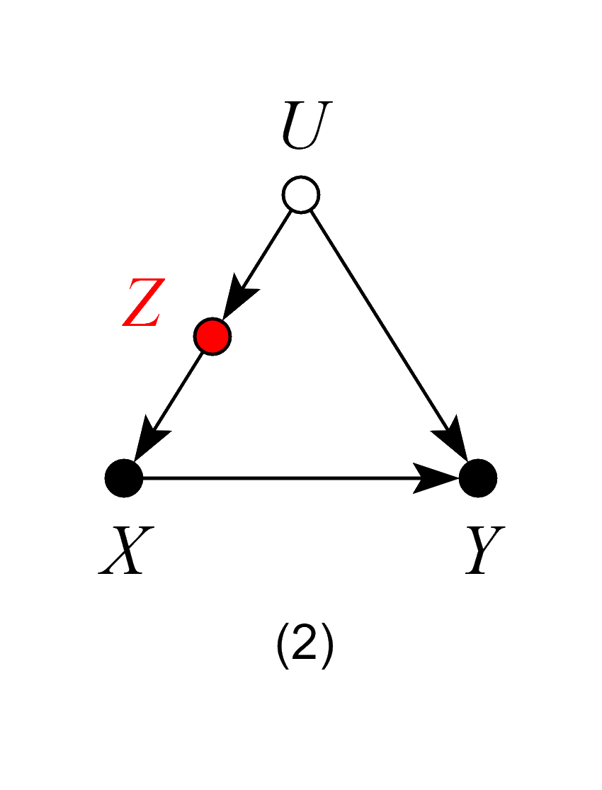
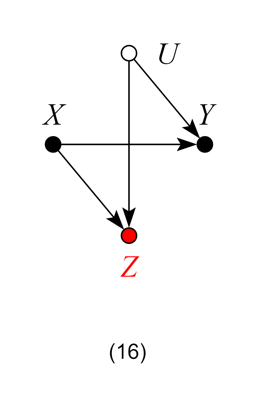
Among these, I consider the causal resolution of Simpson’s paradox (Chapter 22, https://ucla.in/2Jfl2VS) to be one of the crown achievements of CI. The paradox lays bare the core differences between causal and statistical thinking, and its resolution brings an end to a century of debates and controversies by the best philosophers of our time. It is also related to Lord’s Paradox (see https://ucla.in/2YZjVFL) − a qualitative version of Simpson’s Paradox which became a focus of endless debates with statisticians and trialists throughout 2022 (on Twitter @yudapearl). I often cite Simpson’s paradox as a proof that our brain is governed by causal, not statistical, calculus.
This question − causal or statistical brain − is not a cocktail party conversation but touches on the practical question of choosing an appropriate language for casting the knowledge necessary for commencing any CI exercise. Philip Dawid − a proponent of counterfactual-free statistical languages − has written a critical essay on the topic (https://www.degruyter.com/document/doi/10.1515/jci-2020-0008/html?lang=en) and my counterfactual-based rebuttal, https://ucla.in/3bXCBy3, clarifies the issues involved.
(2) The second forum of inter-disciplinary discussions can be found in a special issue of the Journal Observational Studies, https://muse.jhu.edu/pub/56/article/867085/pdf (edited by Ian Shrier, Russell Steele, Tibor Schuster and Mireille Schnitzer) in a form of interviews with Don Rubin, Jamie Robins, James Heckman and myself.
In my interview, https://ftp.cs.ucla.edu/pub/stat_ser/r523.pdf, I compiled aspects of CI that I normally skip in scholarly articles. These include historical perspectives of the development of CI, its current state of affairs and, most importantly for our purpose, the lingering differences between CI and other frameworks. I believe that this interview provides a fairly concise summary of these differences, which have only intensified in 2022.
Most disappointing to me are the graph-avoiding frameworks of Rubin, Angrist, Imbens and Heckman, which still dominate causal analysis in economics and some circles of statistics and social science. The reasons for my disappointments are summarized in the following paragraph:
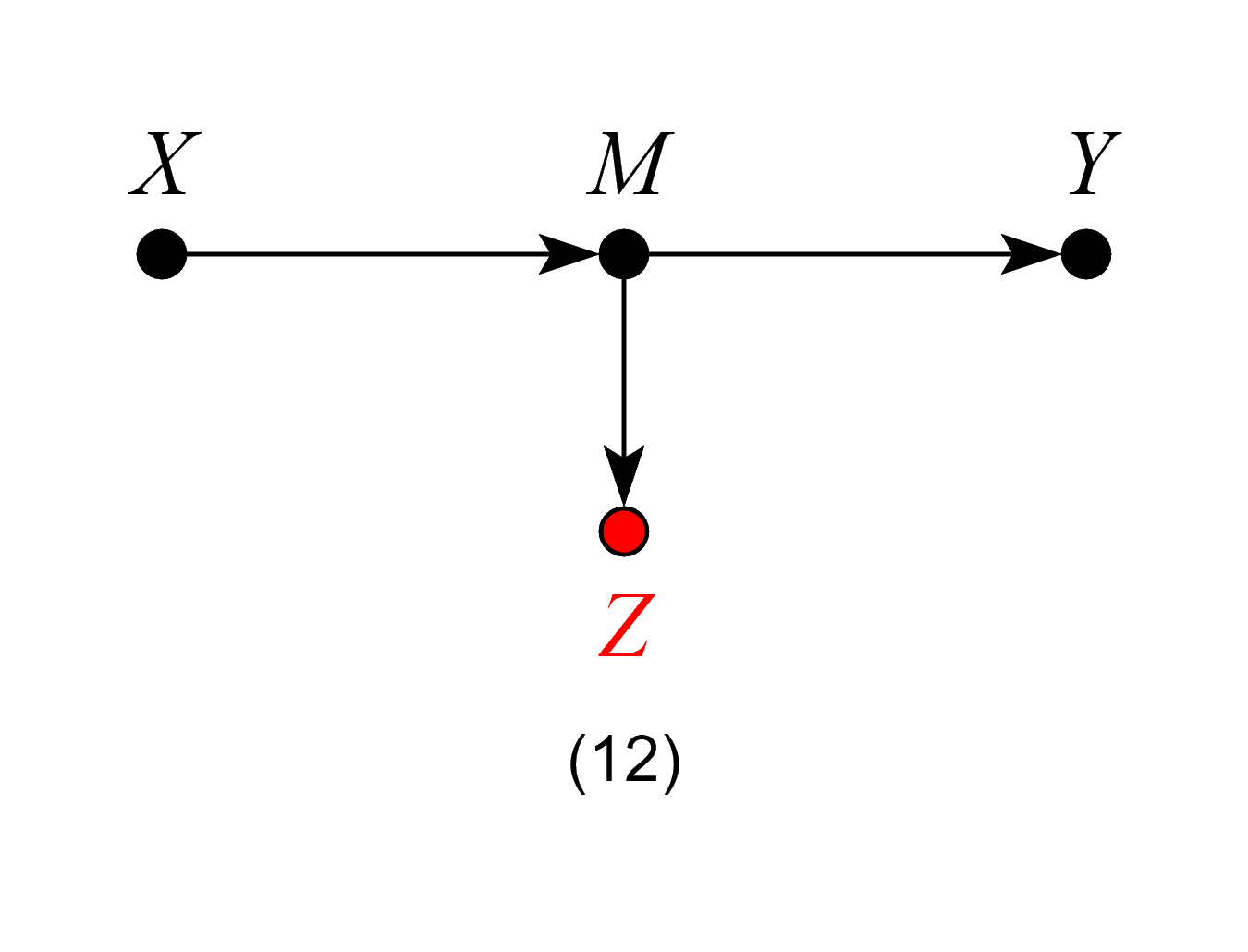
Graphs are new mathematical objects, unfamiliar to most researchers in the statistical sciences, and were of course rejected as “non-scientific ad-hockery” by top leaders in the field [Rubin, 2009]. My attempts to introduce causal diagrams to statistics [Pearl, 1995; Pearl, 2000] have taught me that inertial forces play at least as strong a role in science as they do in politics. That is the reason that non-causal mediation analysis is still practiced in certain circles of social science [Hayes, 2017], “ignorability” assumptions still dominate large islands of research [Imbens and Rubin, 2015], and graphs are still tabooed in the econometric literature [Angrist and Pischke, 2014]. While most researchers today acknowledge the merits of graph as a transparent language for articulating scientific information, few appreciate the computational role of graphs as “reasoning engines,” namely, bringing to light the logical ramifications of the information used in their construction. Some economists even go to great pains to suppress this computational miracle [Heckman and Pinto, 2015; Pearl, 2013].
My disagreements with Heckman go back to 2007 when he rejected the do-operator for metaphysical reasons (see https://ucla.in/2NnfGPQ#page=44) and then to 2013, when he celebrated the do-operator after renaming it “fixing” but remained in denial of d-separation (see https://ucla.in/2L8OCyl). In this denial he retreated 3 decades in time while castrating graphs from their inferential power. Heckman’s 2022 interview in Observational Studies continues his on-going crusade to prove that econometrics has nothing to learn from neighboring fields. His fundamental mistake lies in assuming that the rules of do-calculus lie “outside of formal statistics”; they are in fact logically derivable from formal statistics, REGARDLESS of our modeling assumptions but (much like theorems in geometry) once established, save us the labor of going back to the basic axioms.
My differences with Angrist, Imbens and Rubin go even deeper (see https://ucla.in/36EoNzO), for they involve not merely the avoidance of graphs but also the First Law of Causal Inference (https://ucla.in/2QXpkYD) hence issues of transparency and credibility. These differences are further accentuated in Imbens’s Nobel lecture https://onlinelibrary.wiley.com/doi/pdf/10.3982/ECTA21204 which treats CI as a computer science creation, irrelevant to “credible” econometric research. In https://ucla.in/2L8OCyl, as well as in my book Causality, I present dozens of simple problems that economists need, but are unable to solve, lacking the tools of CI.
It is amazing to watch leading researchers, in 2022, still resisting the benefits of CI while committing their respective fields to the tyranny of outdatedness.
To summarize, 2022 has seen an unprecedented upsurge in CI popularity, activity and stature. The challenge of harnessing CI tools to solve critical societal problems will continue to inspire creative researchers from all fields, and the aspirations of advancing towards human-level artificial intelligence will be pursued with an accelerated pace in 2023.
Wishing you a productive new year,
Judea