A Crash Course in Good and Bad Control
Carlos Cinelli, Andrew Forney and Judea Pearl
Update: check the updated and extended version of the crash course here.
Introduction
If you were trained in traditional regression pedagogy, chances are that you have heard about the problem of “bad controls”. The problem arises when we need to decide whether the addition of a variable to a regression equation helps getting estimates closer to the parameter of interest. Analysts have long known that some variables, when added to the regression equation, can produce unintended discrepancies between the regression coefficient and the effect that the coefficient is expected to represent. Such variables have become known as “bad controls”, to be distinguished from “good controls” (also known as “confounders” or “deconfounders”) which are variables that must be added to the regression equation to eliminate what came to be known as “omitted variable bias” (OVB).
Recent advances in graphical models have produced a simple criterion to distinguish good from bad controls, and the purpose of this note is to provide practicing analysts a concise and visible summary of this criterion through illustrative examples. We will assume that readers are familiar with the notions of “path-blocking” (or d-separation) and back-door paths. For a gentle introduction, see d-Separation without Tears.
In the following set of models, the target of the analysis is the average causal effect (ACE) of a treatment X on an outcome Y, which stands for the expected increase of Y per unit of a controlled increase in X. Observed variables will be designated by black dots and unobserved variables by white empty circles. Variable Z (highlighted in red) will represent the variable whose inclusion in the regression is to be decided, with “good control” standing for bias reduction, “bad control” standing for bias increase and “netral control” when the addition of Z does not increase nor reduce bias. For this last case, we will also make a brief remark about how Z could affect the precision of the ACE estimate.
Models
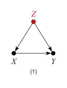
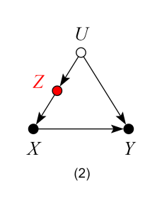
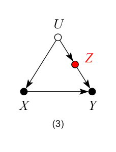
Models 1, 2 and 3 – Good Controls
In model 1, Z stands for a common cause of both X and Y. Once we control for Z, we block the back-door path from X to Y, producing an unbiased estimate of the ACE.
In models 2 and 3, Z is not a common cause of both X and Y, and therefore, not a traditional “confounder” as in model 1. Nevertheless, controlling for Z blocks the back-door path from X to Y due to the unobserved confounder U, and again, produces an unbiased estimate of the ACE.
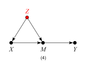
Models 4, 5 and 6 – Good Controls
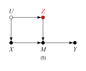
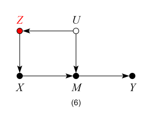
When thinking about possible threats of confounding, one needs to keep in mind that common causes of X and any mediator (between X and Y) also confound the effect of X on Y. Therefore, models 4, 5 and 6 are analogous to models 1, 2 and 3 — controlling for Z blocks the backdoor path from X to Y and produces an unbiased estimate of the ACE.
Model 7 – Bad Control
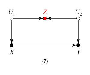
We now encounter our first “bad control”. Here Z is correlated with the treatment and the outcome and it is also a “pre-treatment” variable. Traditional econometrics textbooks would deem Z a “good control”. The backdoor criterion, however, reveals that Z is a “bad control”. Controlling for Z will induce bias by opening the backdoor path X ← U1→ Z← U2→Y, thus spoiling a previously unbiased estimate of the ACE.
Model 8 – Neutral Control (possibly good for precision)
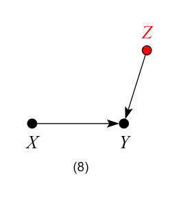
Here Z is not a confounder nor does it block any backdoor paths. Likewise, controlling for Z does not open any backdoor paths from X to Y. Thus, in terms of bias, Z is a “neutral control”. Analysis shows, however, that controlling for Z reduces the variation of the outcome variable Y, and helps improve the precision of the ACE estimate in finite samples.
Model 9 – Neutral control (possibly bad for precision)
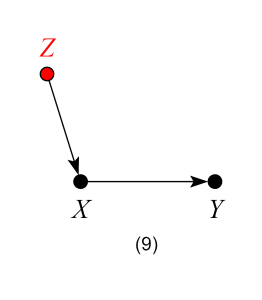
Similar to the previous case, here Z is “neutral” in terms of bias reduction. However, controlling for Z will reduce the variation of treatment variable X and so may hurt the precision of the estimate of the ACE in finite samples.
Model 10 – Bad control
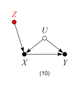
We now encounter our second “pre-treatment” “bad control”, due to a phenomenon called “bias amplification” (read more here). Naive control for Z in this model will not only fail to deconfound the effect of X on Y, but, in linear models, will amplify any existing bias.
Models 11 and 12 – Bad Controls
If our target quantity is the ACE, we want to leave all channels through which the causal effect flows “untouched”.
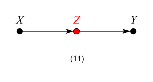
In Model 11, Z is a mediator of the causal effect of X on Y. Controlling for Z will block the very effect we want to estimate, thus biasing our estimates.
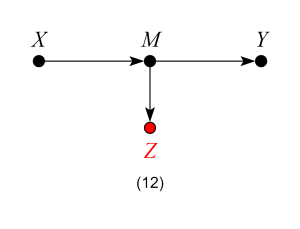
In Model 12, although Z is not itself a mediator of the causal effect of X on Y, controlling for Z is equivalent to partially controlling for the mediator M, and will thus bias our estimates.
Models 11 and 12 violate the backdoor criterion, which excludes controls that are descendants of the treatment along paths to the outcome.
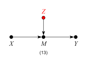
Model 13 – Neutral control (possibly good for precision)
At first look, model 13 might seem similar to model 12, and one may think that adjusting for Z would bias the effect estimate, by restricting variations of the mediator M. However, the key difference here is that Z is a cause, not an effect, of the mediator (and, consequently, also a cause of Y). Thus, model 13 is analogous to model 8, and so controlling for Z will be neutral in terms of bias and may increase precision of the ACE estimate in finite samples.
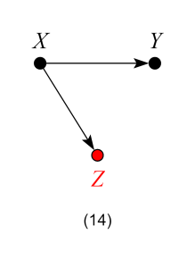
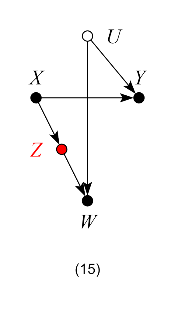
Model 14 – Neutral controls (possibly helpful in the case of selection bias)
Contrary to econometrics folklore, not all “post-treatment” variables are inherently bad controls. In models 14 and 15 controlling for Z does not open any confounding paths between X and Y. Thus, Z is neutral in terms of bias. However, controlling for Z does reduce the variation of the treatment variable X and so may hurt the precision of the ACE estimate in finite samples. Additionally, in model 15, suppose one has only samples with W = 1 recorded (a case of selection bias). In this case, controlling for Z can help obtaining the W-specific effect of X on Y, by blocking the colliding path due to W.
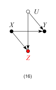
Model 16 – Bad control
Contrary to Models 14 and 15, here controlling for Z is no longer harmless, since it opens the backdoor path X → Z ← U → Y and so biases the ACE.
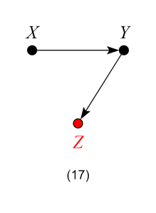
Model 17 – Bad Control
Here, Z is not a mediator, and one might surmise that, as in Model 14, controlling for Z is harmless. However, controlling for the effects of the outcome Y will induce bias in the estimate of the ACE, making Z a “bad control”. A visual explanation of this phenomenon using “virtual colliders” can be found here.
Model 17 is usually known as a “case-control bias” or “selection bias”. Finally, although controlling for Z will generally bias numerical estimates of the ACE, it does have an exception when X has no causal effect on Y. In this scenario, X is still d-separated from Y even after conditioning on Z. Thus, adjusting for Z is valid for testing whether the effect of X on Y is zero.
This is very helpful, thank you so much!
One question: can we draw a causal link from a variable from period t to a variable in t-1? Normally present variables would not affect a variable from the past, but what if these variables measure stock?
i.e.: Total population of 2000 and Total employment of 1999. I was about to use the second one as a control, assuming there is no causal path from 2000 to 1999. But is it weird to consider that it may have, as the stock of 1999 reflects a lot of the 2000 stock value?
Comment by Rubens — September 24, 2019 @ 3:59 pm