Flowers of the First Law of Causal Inference
Flower 1 — Seeing counterfactuals in graphs
Some critics of structural equations models and their associated graphs have complained that those graphs depict only observable variables but: “You can’t see the counterfactuals in the graph.” I will soon show that this is not the case; counterfactuals can in fact be seen in the graph, and I regard it as one of many flowers blooming out of the First Law of Causal Inference (see here). But, first, let us ask why anyone would be interested in locating counterfactuals in the graph.
This is not a rhetorical question. Those who deny the usefulness of graphs will surely not yearn to find counterfactuals there. For example, researchers in the Imbens-Rubin camp who, ostensibly, encode all scientific knowledge in the “Science” = Pr(W,X,Y(0),Y(1)), can, theoretically, answer all questions about counterfactuals straight from the “science”; they do not need graphs.
On the other extreme we have students of SEM, for whom counterfactuals are but byproducts of the structural model (as the First Law dictates); so, they too do not need to see counterfactuals explicitly in their graphs. For these researchers, policy intervention questions do not require counterfactuals, because those can be answered directly from the SEM-graph, in which the nodes are observed variables. The same applies to most counterfactual questions, for example, the effect of treatment on the treated (ETT) and mediation problems; graphical criteria have been developed to determine their identification conditions, as well as their resulting estimands (see here and here).
So, who needs to see counterfactual variables explicitly in the graph?
There are two camps of researchers who may benefit from such representation. First, researchers in the Morgan-Winship camp (link here) who are using, interchangeably, both graphs and potential outcomes. These researchers prefer to do the analysis using probability calculus, treating counterfactuals as ordinary random variables, and use graphs only when the algebra becomes helpless. Helplessness arises, for example, when one needs to verify whether causal assumptions that are required in the algebraic derivations (e.g., ignorability conditions) hold true in one’s model of reality. These researchers understand that “one’s model of reality” means one’s graph, not the “Science” = Pr(W,X,Y(0),Y(1)), which is cognitively inaccessible. So, although most of the needed assumptions can be verified without counterfactuals from the SEM-graphs itself (e.g., through the back door condition), the fact that their algebraic expressions already carry counterfactual variables makes it more convenient to see those variables represented explicitly in the graph.
The second camp of researchers are those who do not believe that scientific knowledge is necessarily encoded in an SEM-graph. For them, the “Science” = Pr(W,X,Y(0),Y(1)), is the source of all knowledge and assumptions, and a graph may be constructed, if needed, as an auxiliary tool to represent sets of conditional independencies that hold in Pr(*). [I was surprised to discover sizable camps of such researchers in political science and biostatistics; possibly because they were exposed to potential outcomes prior to studying structural equation models.] These researchers may resort to other graphical representations of independencies, not necessarily SEM-graphs, but occasionally seek the comfort of the meaningful SEM-graph to facilitate counterfactual manipulations. Naturally, they would prefer to see counterfactual variables represented as nodes on the SEM-graph, and use d-separation to verify conditional independencies, when needed.
After this long introduction, let us see where the counterfactuals are in an SEM-graph. They can be located in two ways, first, augmenting the graph with new nodes that represent the counterfactuals and, second, mutilate the graph slightly and use existing nodes to represent the counterfactuals.
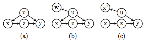
The first method is illustrated in chapter 11 of Causality (2nd Ed.) and can be accessed directly here. The idea is simple: According to the structural definition of counterfactuals, Y(0) (similarly Y(1)) represents the value of Y under a condition where X is held constant at X=0. Statistical variations of Y(0) would therefore be governed by all exogenous variables capable of influencing Y when X is held constant, i.e. when the arrows entering X are removed. We are done, because connecting these variables to a new node labeled Y(0), Y(1) creates the desired representation of the counterfactual. The book-section linked above illustrates this construction in visual details.
The second method mutilates the graph and uses the outcome node, Y, as a temporary surrogate for Y(x), with the understanding that the substitution is valid only under the mutilation. The mutilation required for this substitution is dictated by the First Law, and calls for removing all arrows entering the treatment variable X, as illustrated in the following graph (taken from here).
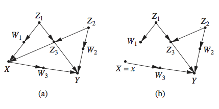
This method has some disadvantages compared with the first; the removal of X’s parents prevents us from seeing connections that might exist between Y_x and the pre-intervention treatment node X (as well as its descendants). To remedy this weakness, Shpitser and Pearl (2009) (link here) retained a copy of the pre-intervention X node, and kept it distinct from the manipulated X node.
Equivalently, Richardson and Robins (2013) spliced the X node into two parts, one to represent the pre-intervention variable X and the other to represent the constant X=x.
All in all, regardless of which variant you choose, the counterfactuals of interest can be represented as nodes in the structural graph, and inter-connections among these nodes can be used either to verify identification conditions or to facilitate algebraic operations in counterfactual logic.
Note, however, that all these variants stem from the First Law, Y(x) = Y[M_x], which DEFINES counterfactuals in terms of an operation on a structural equation model M.
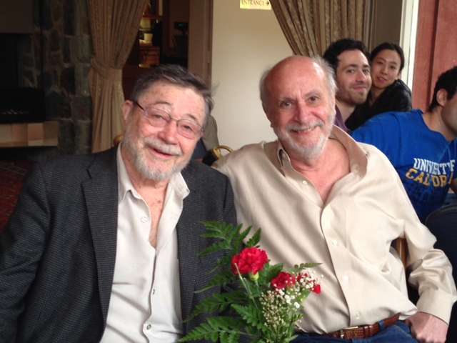
Finally, to celebrate this “Flower of the First Law” and, thereby, the unification of the structural and potential outcome frameworks, I am posting a flowery photo of Don Rubin and myself, taken during Don’s recent visit to UCLA.